Xylem Embolism Meter (Xyl’EM)

Author Affliations

Tete S. Barigah and Herve Cochard INRA, UMR547 PIAF, F-63100 Clermont-Ferrand / Clermont Université, Université Blaise-Pascal, UMR547 PIAF, BP 10448, F-63000 Clermont-Ferrand

Overview

Xyl’EM, xylem embolism meter, is primarily designed for measuring the degree of xylem embolism in vascular plants. The apparatus is an improved version of the Sperry’s one since it measures the water flows with a high precision liquid flowmeter instead of an accurate balance. Thus easy and fast measurements with Xyl’EM can be performed in laboratory as well as in field.

Background

Transpiration at leaf surface pulls water up from the soil into roots and through the xylem conduits of plants. Water in these conduits is under tension which increases as soil moisture content decreases and/or as transpiration rate increases. Water under tension can lead to xylem dysfunction by the breaking of water continuity in the conduit lumen. Embolism results from cavitation phenomenon, a process by which xylem conduits become air-filled and lose their functionality in sap conduction. Embolism rises in plants as a consequence of either freeze-thaw cycles during winter (Sperry and Sullivan 1992)or air-seeding induced by water stress (Sperry et al. 1988a). Embolism can cause a substantial reduction in xylem transport and thus exerts a debilitating influence on plant water status by decreasing its hydraulic conductance. Besides, embolism is one of the most important threats to vascular plants, causing catastrophic xylem dysfunction when a threshold of water stress is passed (Tyree and Sperry, 1988). So far, embolism is commonplace in plants (Milburn, 1991) and native steady state embolism and the related percent loss conductivity (PLC) are assessed by inserting excised stem segments in conductivity apparatus (Cochard 1992; Magnani and Borghetti 1995; Sperry et al. 1987).

The reference -hydraulic’ method for quantifying xylem embolism relied on a conductivity apparatus devised by (Sperry et al. 1988a). This method consists in estimating the hydraulic conductance of a stem segment before and after successive perfusions under pressure with degassed distilled water. The perfusion evacuates or dissolves air contained in the embolized xylem vessels. The initial to final conductance ratio gives a quantitative value of embolism level i.e. its steady state embolism and the related percent loss conductance (PLC). This technique is now wide-spread but remains laborious and delicate as it requires the use of a precision balance, and is unusable in the field.

The following protocol explains how to achieve a stem-segment (root and/or petiole as well) hydraulic conductance per unit pressure gradient measurement with the Xyl’Em.

Materials/Equipment

• Xyl’EM apparatus
• Razor blade
• Computer with a software to power up the Xyl’EM
• Filter of a 0.2 μm filtration membrane (Calyx capsule, Osmonics Inc., Westborough, USA or Polycap 75 AS, Watman)
• Feeding tank (a vacuum resistant Erlenmeyer flask)
• Secondary supply tank (named water basket in the instruction manual)
• Luer tubes and fitting connectors
• Compressed air provider
• Sample manifold

Units, terms, definitions

The hydraulic conductance (k_h, kg s^-1 MPa^-1) is known as the inverse of the hydraulic resistance (k = 1/R) and is the water flow rate (F, kg s^-1) across a plant component divided by the pressure (P, MPa^-1) causing the flow. k_init and k_max stand for initial and maximum conductances.

Native steady state embolism is expressed as

K_h = F/ P/l (1)

Percentage Loss of Conductivity (PLC, %) is calculated from

PLC = 100 (k_max – k_init) / (k_max) (2)

NB. Initial hydraulic conductivity (k_init, kg s^-1 MPa^-1 m), should be determined by measuring the solution flow rate (from the water basket) perfused through the stem segment of l meter long at a pressure drop ( P, MPa) of about 6 kPa.

Procedure

Hook up the Xyl’EM for measuring hydraulic conductance in stem segment

The Xyl’EM requires to be hooked up on the one hand to a computer for running an implemented program to output the conductance data, on the other hand to a set of plastic tubes, a sample manifold and an in-line 0.22 μm-mesh membrane filter holder. To proceed:

1. Lay down the Xyl’EM on a bench between a computer and a basin of tap water
2. Connect the Xyl’EM to the computer via the RS232 wire cable (RS, Xyl’EM front panel)
3. Plug in both the computer and the Xyl’EM to power up them
4. Connect the temperature probe to the Xyl’EM and keep the sensor head emerged in the tap water contained in the water basin
5. Connect the in-line membrane filter holder to the inlet/outlet F connexion ports of the Xyl’EM (see the front panel)
6. Connect the feeding tank to the inlet water port (to fill the inner tank) via a 3-way stopcock using a Luer tube or a Tygon tube (a home made connexion is needed). Always, fill by gravity the inner tank with de-ionized, de-gassed and filtered (0.2 μm) 10 mM KCl l^-1 and 1 mM CaCl₂ l^-1 solution
7. Connect the compressed air provider to the Xyl’Em’s air inlet
8. Connect the water basket to a 3-way stopcock
9. Connect one void of this stopcock to the W.B. (Water Basket) port with a Luer tube
10. Connect the last void of this stopcock to a Luer tube and keep its free ending under the tap water inside the basin
11. Connect the sample manifold to the outlet port with a Luer tube
12. Switch on both the Xyl’EM and the computer
13. Refer to the instruction manual to fulfil the inner tank, the connexion tubings as well as the sample manifold mainly if you are running this operation for the first time
14. Make sure to remove all air bubbles from the water circuitry
15. Insert the samples in the sample manifold
16. The set-up is completed and ready for sample conductance measurements.

Preparing the plant material

Plant material (stem, petiole, mature portion of roots) requires a great care from harvesting to inserting in the sample manifold. The segments must be collected and prepared in such way so as to minimize the introduction of additional air bubbles into the xylem (see (Sperry et al. 1988a) for more details). When possible, feel free to spray water over the foliage of the target shoot before cutting or remove the leaves from the shoot prior to pruning.

1. Cut a shoot as long as possible from the mother plant
2. Wrap it in a wet black plastic bag or keep the cut end inside tap water
3. At least a piece of 0.15 m long should be removed under water from the cut end of each shoot and discarded. When focusing on petioles, they should be cut under water.

Software set up

1. Turn on the computer connected to the Xyl’EM and run the program that power up the Xyl’EM
2. Select the “set up” option to access the configuration options
3. Customize this page according to the type of flow-meter in duty; provide the calibration coefficient for the flow-meter as well as for the temperature and pressure probes. Make sure to select the right flow-meter (Int/Ext) if your Xyl’Em is released with these options
4. Select the units of the probes
5. Tick the automatic or manual option accordingly to your requirement
6. Fill in options related to the scrutinising time, the number of samples and number of -flushes’
7. Valid your selections
8. Before leaving this page, tick the “LP” option for dedicating the device for Percent Loss Conductance (PLC) determination. “HP” option must be select for using the device as a High Pressure Flow Meter (HPFM)
9. Switch to the “Measure” window
10. If necessary, one can change here the default scrutinising-time interval, the sample and flush numbers and the options regarding the flow rate, temperature, low and high-pressure.

Measurement processing

Set up the zero flow

This consists in closing the water basket outlet and opening the manifold to vent

1. Turn the first 3-way valve to “Flow”, the second 3-way valve to “0” and the third one to “LP”
2. Click on the offset L-Press button on the computer screen to record the zero low pressure-flow offset
3. Close the manifold vent

Measurement of k_init

1. Turn the 3-way valve (manifold) so that the target sample could be perfused with the solution from the water basket
2. Turn the 3-way valve hooked to the water basket to let its content feeds exclusively the target sample
3. Click on the GO button on the computer screen
4. Acquisition of initial conductance (k_init) starts and its values display automatically in the values window when each scrutinising time is over
5. When the k_init reaches a steady state value, the coloured column turns from red or orange to green
6. Clicking on the OK button on the computer screen leads to stop k_init data acquisition. In the meantime, k_init mean and standard deviation values are calculated and displayed in the -stat’ window. Only the k_init-mean value is displayed in the “kinit” column in front of the sample 1 line.
7. Turn the 3-way valve that feeds the first target sample to prevent perfusing inward it
8. Select the next sample as target by allowing the solution from the water basket to flow exclusively through this new target sample
9. Initiate a loop by activating steps 4 to 10 to complete the k_init measurement of this new target sample (sample 2)
10. Go for the same procedures to record k_init value for each of the samples inserted into the manifold

Flushing the samples measured for k_max measurement

1. Close the water basket outlet
2. Turn all the 3-way valves of the samples in the sample manifold to allow water flow through all the samples simultaneously. Keep the vent outlet locked
3. Turn the second 3-way valve on the Xyl’EM front panel to “air” to allow compressed air into the inner tank up to 0.2 MPa maximum. Turn this 3-way valve to “0”
4. Turn the third 3-way valve on the Xyl’EM front panel to “HP” for few seconds to perfuse all the samples with high-pressured solution up to 0.2 MPa maximum
5. Wait for few minutes to allow high pressure relaxation within all the samples. Then, close water entry for all the samples (by turning their 3-way valve) except for the first-target sample

Measurement of k_h

1. Open the water basket outlet to allow exclusively solution flow towards the samples
2. Redo operations from steps 4 to 13
3. Go anew for flushing operations (steps 15-19)

Measurement of k_max

1. Repeat operations related to steps 22 and 23 until k_h does no longer increase.
2. Turn all the 3-way valves on the Xyl’EM front panel to “0”
3. Save the data to an Excel file
4. Remove the samples from the sample manifold and proceed to measurements of their length and the diameter of the proximal end.

Other resources

Notes and troubleshooting tips

• If the plant material is too thin, you can put Teflon tape around it to fit the insert tubing (sample manifold)
• During the first flush, take the sample manifold out of the water to check for leaks around the insertion points.

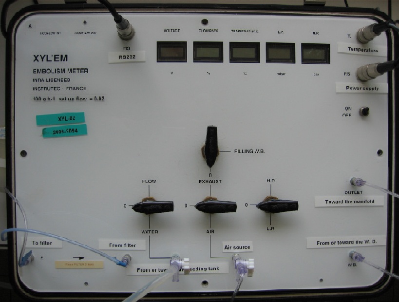
Fig 1: Front panel of the Xyl’Em

Fig 2: Close up on front panel

Fig 3: Configuration for the 3-way valves at the starting point (zero flux)

Fig 4: Poplar stem-segments inserted into the Manifold, with the temperature probe and the free end of the Luer tube under water

Fig 5: Configuration of the 3-way valves for setting up the zero flow measurement

Fig 6: Configuration of the 3-way valve of the water basket inlet and outlet during the set up of the zero flow measurement

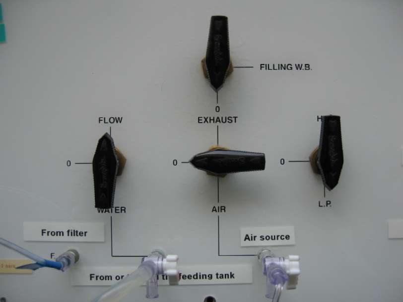
Fig 7: Configuration of the 3-way valves for setting up the k_init, k_max and k_h measurements

Fig 8: Configuration of the 3-way valve of the water basket inlet and outlet during the set up of the k_init, k_max and k_h measurements

Fig 9: Configuration of the 3-way valves for filling up the inner tank (from the feeding tank)

Fig 10: Configuration of the 3-way valves for filling up the water basket

Fig 11: Configuration of the 3-way valves for storing compressed air inside the inner tank

Fig 12: Configuration of the 3-way valves for flushing the samples to up to 0.2 MPa

Links to resources and suppliers

Flow measurement:

• Principle: Thermal mass flow measurement
• Measuring range: 0.1-5 g/h, 0.2-10 g/h, 0.4-20g/h, 1-50 g/h, 2-100 g/h H2O (to be specified on the order).
• Accuracy: + / – 1% full scale
• Range span: 1 to 50

Low pressure generation and measurement:

• Principle: Water column
• Measuring range: 1 .. 7 kPa typ, (10 kPa max)
• Accuracy: +/- 0.2 kPa

High pressure generation and measurement:

• Principle: Pressurised vessel
• Measuring range: up to 3 bar typ, 7 bar max.
• Accuracy: +/- 1 % full scale

Temperature

• Sensor: Pt100 probe
• Measuring range: 0� C to 50� C
• Accuracy: +/- 0.2 � C

Water supply:

High pressure:

• Vessel capacity: 1 litre
• Max vessel pressure: 3 bars, (7 bars possible if filter is removed).

Low pressure:

• Vessel capacity: 100 ml
• Max vessel pressure: 1 meter water high
• Water filtration: 0.2 m.

Mechanical characteristics

• Suitcase: IP65
• Dimension: 461x347x206 mm
• Weight (empty vessel): 10 kg

Electrical characteristics

• Power supply: 12 Vdc
• Consumption: 900 mA
• Electrical connection: Din 3 pins

Computer connection (option):

• Analog to digital conversion (15 bits resolution) and RS232 interface for data transfer to a computer.
• XYL’EM software for DOS and windows environments. This software collects the data, calculates the corrections and determines embolism factor.
  

Literature references

Cited references

Cochard H (1992) Vulnerability of several conifers to air embolism. Tree Physiology 11, 73-83

Magnani F, Borghetti M, (1995) Interpretation of seasonal changes of xylem embolism and plant hydraulic resistance in Fagus sylvatica. Plant Cell and Environment 18, 689-696

Milburn JA (1991) Cavitation and embolism in xylem conduits. In “Physiology of trees“, A. S. Raghavendra (editor), pp. 163-174. J Wiley & Sons, New York, 509 p

Sangsing K, Kasemsap P, Thanisawanyangkura S, Sangkhasila K, Gohet E, Thaler P, Cochard H (2004) Xylem embolism and stomatal regulation in two rubber clones (Hevea brasiliensis Muell. Arg.). Trees-Structure and Function 18, 109-114

Sperry JS, Donnelly JR, Tyree MT (1988a) Seasonal occurrence of xylem embolism in sugar maple (Acer saccharum). American Journal Botany 75, 1212-1218

Sperry JS, Donnelly JR, Tyree MT (1988b) A method for measuring hydraulic conductivity and embolism in xylem. Plant, Cell and Environment 11, 35-40

Sperry JS, Holbrook NM, Zimmermann MH, Tyree MT (1987) Spring filling of xylem vessels in wild grapevine. Plant Physiology 83, 414-417

Sperry JS, Sullivan JEM (1992) Xylem embolism in response to freeze-thaw cycles and water stress in ring-porous, diffuse-porous, and conifer species. Plant Physiology 100, 605-613

Other Literature references

Cochard H, Bodet C, Ameglio T, Cruiziat P (2000) Cryo-scanning electron microscopy observations of vessel content during transpiration in walnut petioles. Facts or artifacts Plant Physiology 124, 1191-1202

Cochard H, Coll L, Le Roux X, Améglio T (2002) Unraveling the effects of plant hydraulics on stomatal conductance during water stress in walnut. Plant Physiology 128, 282-290

Cochard H, Herbette S, Barigah T, Badel E, Ennajeh M, Vilagrosa A (2010) Does sample length influence the shape of xylem embolism vulnerability curves A test with the Cavitron spinning technique. Plant Cell and Environment 33, 1543-1552

Cruiziat P, Cochard H, Améglio T (2002) The hydraulic architecture of trees: main concepts and results. Annals of Forest Sciences 59, 723-752

Cochard H (2002) Xylem embolism and drought-induced stomatal closure in maize. Planta 215, 466-471

Espino S, Schenk H J (2011) Mind the bubbles: achieving stable measurements of maximum hydraulic conductivity through woody plant samples. Journal of Experimental Botany 62, 1119-1132

Lovisolo C, Tramontini S (2010) Methods for assessment of hydraulic conductance and embolism extent in grapevine organs. In “Methodologies and results in grapevine research”, pp 71-85, doi:10.1007/978-90-481-9283-0_6

Tyree MT, Cochard H (2003) Vessel content of leaves after excision: a test of the Scholander assumption. Journal of Experimental Botany 54, 2133-2139

Tyree MT, Cochard H, Cruiziat P (2003) The water-filled versus air-filled status of vessels cut open in air: The ‘Scholander assumption’ revisited. Plant Cell and Environment 26, 613-621

Sangsing K, Kasemsap P, Thanisawanyangkura S, Sangkhasila K, Gohet E, Thaler P, Cochard H (2004) Xylem embolism and stomatal regulation in two rubber clones (Hevea brasiliensis Muell. Arg.). Trees, Structure and Function 18, 109-114

Zufferey V, Cochard H, Ameglio T, Spring JL, Viret O (2011) Diurnal cycles of embolism formation and repair in petioles of grapevine (Vitis vinifera cv. Chasselas). Journal of Experimental Botany 62 (11), 3885-3894. doi:10.1093/jxb/err081

Health, safety & hazardous waste disposal considerations

!

Species on which this protocol has been used

Family	Genus	Species	Growth forms	Kind of setting	Related references
Asteraceae	Encelia	farinosa Torrey & A. Gray	desert Desert shrub	Lab	Espino and Schenk, 2011
Asteraceae	Helianthus	annuus L.	Herb	Lab	Tyree, Cochard 2003
Betulaceae	Betula	pendula Roth	Temperate tree	Lab	Cochard et al, 2010
Betulaceae	Carpinus	betulus L.	Temperate tree	Lab	Cochard et al, 2010
Betulaceae	Populus	tremula L.	Temperate tree	Lab	Barigah, unpublished data
Euphorbiaceae	Hevea	brasiliensis Muell. Arg.	Tropical forest tree	Lab	Sangsinget al, 2004; Cochard et al, 2010
Fabaceae	Robinia	pseudoacacia L.	Tree	Lab	Cochard et al, 2010
Fagaceae	Castanea	sativa Mill.	Temperate tree	Lab	Cochard et al, 2010
Fagaceae	Fagus	sylvatica L.	Temperate tree	Lab	Barigah, unpublished data
Fagaceae	Quercus	petraea Matt.Liebl	Temperate tree	Lab	Chevalier, unpublished data
Fagaceae	Quercus	robur L.	Temperate tree	Lab	Chevalier, unpublished data
Juglandaceae	Juglans	regia L.	Temperate tree	Lab	Cochard et al, 2000, 2002; Cruiziat et al, 2002 ; Tyree et al 2003
Lauraceae	Laurus	nobilis L.	Mediterranean evergreen tree	Lab	Espino and Schenk, 2011
Oleaceae	Fraxinus	excelsior L.	Temperate tree	Lab	Cochard et al, 2010
Oleaceae	Olea	europaea L.	Mediterranean tree	Lab	Cochard et al, 2010
Poaceae	Zea	mays	herb	Lab	Cochard 2002
Ranunculaceae	Clematis	vitalba L.	Vine	Lab	Cochard et al, 2010
Rosaceae	Prunus	persica L. Batsch	Temperate tree	Lab	Cochard et al, 2010
Sapindaceae	Acer	platanoides L.	Temperate tree	Lab	Tyree et al, 2003
Vitaceae	Vitis	vinifera L.	Vine	Lab	Lovisolo and Tramontini 2010; Cochard et al, 2010 ; Zufferey et al, 2011