Protocol

 

Authors

Robert Pearcy, Remko Duursma, and Daniel Falster

OVERVIEW

This protocol outlines techniques for mapping the 3D architecture of plants, and for simulating light capture and carbon gain of the digitised specimens using the Yplant software.

Insights

– The adaptive significance of inherent variation in leaf form, shoot and whole-plant architecture (Falster and Westoby 2003; Duursma et al. 2012).

– The adaptive significance of phenotypic plasticity (Valladares and Pearcy 1998).

– The influence of different light regimes on light interception and potential carbon gain (Lusk et al. 2011).

BACKGROUND

Y-plant is a 3-dimensional (3D) crown architecture model for analysis of light capture and carbon gain of plants, with special attention to the geometry of the crown and self shading. Yplant uses a 3D reconstruction of an individual plant (or part thereof) combined with a hemispherical canopy photo to calculate leaf display, diffuse light absorption over all directions, and direct light absorption accounting for the position of the sun. Light interception data are combined with a leaf photosynthesis model to estimate carbon assimilation. The model is described in Pearcy and Yang (1996) and has been used in a number of publications, to study species differences in light interception and carbon assimilation, to examine the optimality of allocation, and for studying the consequences of architectural plasticity (see Publications using Yplant (Part II, below). Subsequent enhancements to the model include a more sophisticated Farquhar-von Cammerer-Berry (1980) type photosynthesis model, a leaf energy balance sub-model for computing leaf temperatures and transpiration rates, a hydraulic sub-model for mapping water flow and water potentials and a photoinhibition sub-model. Collection of input data for Yplant was initially done by hand, which was very time consuming. Later, Falster and Westoby (2003) developed a much faster method based on 3D digitising technology to Yplant.

The features and limitations of Yplant are:

• Can handle up to 10000 nodes (leaves). The limitation is the effort required to obtain the necessary geometric data for this many nodes.
• Up to 20 different leaf types differing in shape, physiology, or both can be specified.
• A range of different phyllotaxes can be simulated.
• Leaves are modelled as flat surfaces but folded and curved leaves can be approximated in limited circumstances by combining flat surfaces.
• The ray tracing simulation does not take into account beam scattering or reflection back to other leaves. We assume that an intercepted beam is reduced by the leaf reflectance and absorptance, before passing directly through to possibly be intercepted by another leaf.
• Evaluates the capture of both direct and diffuse light with or without a canopy file where an overstory canopy or other landscape features such as a slope obscures part of the sky.
• Assumes that the entire crown is in the same light environment rather than the much more complex reality of considerable spatial variation across crowns due to penumbral effects.
• Several different estimates of light capture efficiency are produced.
• Leaf by leaf simulations of photosynthetic performance, energy balance, stomatal conductance and transpiration can be run and allow scaling from leaf to whole plant performance.
• Input files can be modified using auxiliary programs to examine the effects of phyllotaxy, internode length, leaf angle, etc. on crown performance.

The following briefly describes the necessary measurements and how to run Y-plant. See Pearcy and Yang (1996) for information on the equations and the underlying assumptions.

DOWNLOAD

You can download the Yplant software here: Yplant3.3-zip or via the attachment at the base of this page.

Yplant3.3 is an update of Yplant 3.2 that corrects three problems. Comparisons of the computed displayed leaf area between Yplant 3.2 and YplantQMC developed by Remko Duursma and Mik Cieslak revealed a systematic underestimation of the displayed leaf area that depended on the number of leaves, the sampling gridsize and possibly other factors such as leaf shape. At small gridsizes, which give a denser sampling of the sunlit and shaded leaf area, the error was <1% for plants with up to 300 leaves and only 2.6% for a plant with 695 leaves. Larger gridsizes however result in larger underestimations. The changes in Yplant given below result in whole-plant displayed leaf area values within ∓ 0.5% of those given by YplantQMC.

In Y-plant3.3 the following changes were made:

1. The sampling algorithm was modified to eliminate the negative bias in the displayed leaf area.

2. Gridsize is now set to a value small enough to minimize sampling errors and can no longer be changed in the parameters popup window by the user. The penalty is that Y-plant runs slower but with the fast processors in today’s PCs only 4 min are required for the diffuse light simulation, the slowest step in Yplant, with a plant having 695 leaves. The ability to vary the gridsize was originally important in early Yplant versions that were run on much slower PCs but is unnecessary now.

3. The computation of the leaf area factor from the leaf edge coordinates was modified. The original code underestimated the correct value for a square leaf by 2% but gave correct values for actual leaf shapes. The modified version now give the correct value for all leaves, including square leaves. The leaf area factor is used to scale the area of a leaf from its length assuming that the shape is constant.

This will likely be the last update of Yplant. Increasingly, there are compatibility issues between Borland Delphi, the language used for Y-plant, and Windows Vista/7/8 (see section 10.1.4).

The development by Remko Duursma and Mik Cieslak of a powerful new implementation of Y-plant (YplantQMC) using the R software package provides a path for further enhancements. It incorporates most of the important functions of Y-plant with a more sophisticated ray tracing model that accounts for scattering due to reflection and transmission of light through leaves. It is also more easily extensible by users. For example, different photosynthesis or other physiological models can be incorporated. It is compatible with legacy Yplant input files. We recommend migrating to it.

UNITS, TERMS, DEFINITIONS

The following are measures of light capture efficiency that can be computed from Yplant output. Input variables and definitions in the description of the measurement procedure.

• Absorption Efficiency (E_a)

 

dimensionless

The units for PFD are μmol photons m^-2s^-1

• Effective leaf area ratio (LAR_e)

 

This measure of efficiency expresses how effectively biomass is invested for light capture. Photon flux (PF) has the units of μmol photons s^-1. It requires measurement of the above-ground plant mass.

• Projection Efficiency (E_p)

 

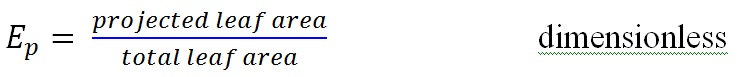
This measure expresses the effects of leaf angles on light interception from a specific direction. In Yplant it can be computed for each of 160 sky sectors and also for specific solar positions along a solar track.

• Display efficiency (E_d)

 

This measure is the ratio of the projected leaf area that is visible from a particular direction to the total leaf area. It expresses how the combination of leaf angles and self shading influence light capture from a particular direction. The fraction of the leaf area that is self shaded within the crown is equal to E_p–E_d. Other indices of light capture efficiency such as the ratio of displayed to total leaf area, averaged over the entire sky hemisphere (the Silhouette to Total Area Ratio: STAR) can be computed from E_d.

PROCEDURE

1. The Yplant format

Plants and their growth environment are described using 3 files. The plant file describes the geometrical arrangement of stems, branches, petioles and leaves in the plant. The leaf file describes leaf shape and leaf physiological data. An optional canopy file describes the shading by the surrounding canopy.

1.1. Plant file

The plant file describes the geometrical arrangement of stems, petioles and leaves in the plant. The node is the fundamental unit in Y-plant. A node can have three objects attached to it:

1. a leaf (with a petiole)
2. a stem
3. a branch

Note that the stem or branch segments defined at a particular node are those extending from the node, not the segment connecting the node to its mother node. A node is connected back to the rest of a plant via a stem or branch segment to a mother node. The properties of this stem or branch segment are defined at the mother node.

Each node may be connected to a single leaf. For opposite leaves, a separate node is created for the second leaf. The internode extending to the second leaf of the pair is given a negligible length (0.1mm) thereby simulating an opposite leaf. Similarly, species with compound leaves can be mapped by treating the rachis as a branch.

An example plant is included below, PlantFile.p (or download attachment at base of page). Each row gives data for a single node. First are the node number (N) and the node that it connects to (the “mother node”, (MN). The next column (ste) specifies whether this node is connected to its mother node by the stem (1) or branch (2). Designation of a particular segment as “stem” or “branch” is arbitrary. It only serves to identify which node is connected to the mother node by which segment. Therefore, a “branch” at one node can (and usually will) become a “stem” at subsequent nodes along the same path. The leaf type (Lt) specifies the type (1,2…) of leaf attached, if any. Unless there are very different leaf shapes or if different leaves (old versus young for example) have different physiological characteristics, the leaf type is 1, or 0 if there is no leaf at the node. The next four columns give the Azimuth (Az), Angle from horizontal (An), Length (L) and diameter (D) of the stem segment protruding from the node. The following four columns give similar data for a branch segment. Note that a single node can only have one branch and one stem. If you are mapping a plant with whorled branches, you will need to create a separate node for each new branch. Columns 14-16 likewise give the Azimuth (Az), Angle from horizontal (An), Length (L) and diameter (D) of the petiole. The last four columns then describe the orientation of the leaf surface. Or is the orientation (azimuth) of the midrib, while Az and An are the azimuth and angle from horizontal for normal vector to the leaf surface. L is leaf length, measured along the midrib.

Note that all length and diameter measurements are in millimetres. Azimuths angles are defined relative to true north. It is important to remember that the compass declination must therefore be taken into account, either by adjusting the compass or by correcting all the measurements later.

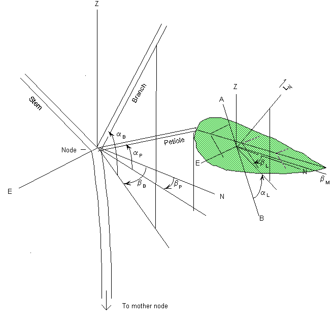
Figure 1 defines the angles required for Y-plant. E, N and Z are the East, North and zenith directions, respectively. is an angle from horizontal. is an azimuth (0-360°). the subscripts B, P, L, M refer to branch, petiole, leaf and midrib, respectively. LN is the leaf surface normal, the leaf angle is measured along the line A-B. ℼ_M is the leaf orientation; _L is the leaf azimuth.

1.2. Leaf file

The leaf file contains a description of the leaf shape as well as leaf physiological parameters. A document descirbing the format (Leaf_example.doc) and examples of working files LeafFile.l and LeafFile.lf are included as attachments to this page.

The leaf shape component consists of points mapped around the leaf edge, starting with the base of the petiole. The number of points needed for any accurate description will depend on the leaf shape. This figure shows the position of 25 points.

 

In Yplant, leaves are treated as flat surfaces but it is possible under limited circumstances to model more complex folded or curved leaves. Leaves folded along the midrib can be modelled as two abutted surfaces, each as a different leaf type (Falster and Westoby 2003). Curved leaves such as found in many grasses can be modelled by treating the midrib as a stem with a series of nodes and internodes giving the curvature, with surfaces attached at each node (See Valladares et al, 2001). Again, the surfaces can be of different shapes with each being a different leaf type to account for example for the tip versus middle segments. The major limitation treating curved or folded leaves is the more complex data collection. Thus it is best applied to relatively small plants. With some creativity many plants not conforming to the basic Y-plant model can be successfully reconstructed.

Following the coordinates of the leaf outline are the physiological parameters necessary to model leaf photosynthesis. There are two different file formats: one with an extension .L that contains parameters necessary for the Thornley-Johnson (T-J) rectangular hyperbola light response curve model and another with the extension .LF that additionally has the parameters for the Farquhar- von Caemmerer -Berry photosynthesis (FvCB) model. The parameters required for the T-J model are the light saturated assimilation rate, the photon yield the curvature factor that determines the sharpness of the transition between light limitation and saturation, the day respiration rate, and the leaf absorptance and transmittance important in light capture. A .LF file contains all these parameters plus the maximum rate of carboxylation (V_cmax) and electron transport (J_max) and the photon yield of electron transport that are required for the FvCB model. Multiple leaf types differing in shape or physiology are included by concatenating this basic format for each.

The plant and leaf file can also be used with allometric equations for mass, established from other nearby plants, to non-destructively estimate above-ground, whole-plant mass. This is useful for understanding the relationships between light capture and the allocation of biomass.

It is important to map several leaves from each plant, and use a unique averaged shape to populate the nodes of each individual plant. Even in species lacking obvious heterophyIly, it is difficult to appreciate how variable leaf shape is both within and between plants, until it’s actually measured. If only a single apparently “representative” leaf is used for all simulations with multiple plants of a given, the total foliage area computed by YPLANT can differ by up to 35% from direct measurements made with a leaf area meter. Averaging in Excel is straightforward for leaves with entire margins. Averaging the shapes of leaves with small teeth involves a trivial loss of information (the teeth are smoothed out), but lobed leaves are more problematic. In the latter case, dimensional criteria might be used to select a modal shape.

1.3 The light environment

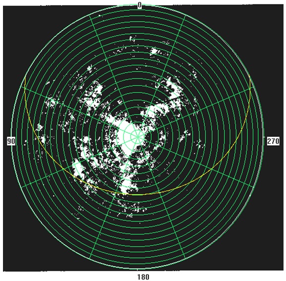
Yplant either assumes that either the plant is in the open and not shaded by surrounding vegetation or utilizes “fisheye” or hemispherical photos taken over the plant to estimate the effects of shading from the surrounding vegetation on light interception and photosynthesis. Both approaches use a solar radiation model to compute the direct and diffuse PPFD and the azimuth and elevation angle of the direct beam, and the diffuse skylight distribution. For the shading effects, the photos need to be processed using an image analysis program. Yplant can accept input files created by either HemiView marketed by Delta-T, or CANOPY developed by Rich (1990). Other hemispherical analysis programs are available and although they have not been tested it seems likely that the necessary data from at least some them could be reformatted to be read by Yplant. Details of the theory, photographic methodology, and the photo analysis can be found in http://en.wikipedia.org/wiki/Hemispherical_photography, Pearcy (1989) and Rich (1990). An example of a hemispherical photo taken with a Nikon FC-E8 fisheye lens on a Coolpix 990 digital camera is shown below. Canopy gaps are white while the foliage is black. The green overlay is from HemiView and shows the sky sectors used in the diffuse light calculations while the yellow line shows a solar track used in the direct light computations.

Files created by CANOPY are text files with the extension .CAN. CANOPY is obsolete but the basic file format may be useful in imputing hemispherical data from other photo analysis programs into Yplant. While .CAN files have many types of data, only two are used by Y-plant. The first is a table derived from partitioning the hemispherical sky into 160 segments. Row 1 and column 1 give the centroids of the sky segments, respectively while the values in each cell are the contribution of the sky segment to the diffuse light at the point of the photo. The second is a list of start and stop times for “sunflecks” created by canopy gaps along a solar track for a specific date. The first table is detected by the label “INDIRECT SITE FACTOR” while the list of sunflecks is detected by the text ‘start end’. An example canopy file Canopy.can with the two essential components is available as an attached file at the base of this wikipage.

Files created by HemiView are in Excel Format. Sheet 1(summary) must contain in cell A1 ‘Summary’ which is necessary to identify whether the file was created by Hemiview 2.1 or alternatively by an earlier version. Earlier versions can be read by Yplant but only the format created by HemiView 2.1 will be presented here. Sheet 2 (Comments) is for notes. Sheet 3 (SkyGap) contains the gap fractions of the 160 sky sectors. Sheet 4 (TimeSer) contains a time series of solar radiation for a specific solar track specified by the day of the year and the latitude. The date and latitude entered in HemiView must match the date and latitude entered in Y-plant. Yplant uses only column A ( time) and D (SunVis, the fraction of the solar disk visible through the gap). When SunVis >0 Yplant detects a “sunfleck” and then computes an average SunVis until SunVis=0 is encountered. This simulates the penumbral effect on sunfleck PFD and gives a more realistic time series of PFDs in the Yplant simulations. The time series should ideally be in 1 min intervals to avoid missing sunflecks >1 min; those <1 min are generally insignificant for assimilation in an understory. The time can be in any standard format supported by Excel since all are read in by Yplant as a general format (day plus decimal fraction of a day). Only the decimal fraction of a day is used. It is important that the exact format be followed. That is for SkyGap the gap fractions must be in cells B6 to I25. For TimeSer the time must start in cell A6 and SunVis in cell D6. An example HemiView file (HemiView.xls) is available as an attached file at the base of this wikipage.

1.4 Creating composite and idealized light environments

.CAN files can be averaged in Excel to develop composite light environments (Falster and Westoby 2003). These are useful for comparing light interception and potential carbon gain of different species in a common light environment (Falster and Westoby 2003). Idealized light environments can be created by manipulating the “INDIRECT SITE FACTOR” table to represent, for example, the centre and margins of tree-fall gaps at different latitudes (Lusk et al. 2011). The hemispherical distribution of canopy openness beneath a tree-fall gap depends on gap diameter and canopy height. The direct light regime beneath the gap depends also on latitude, time of year and cloudiness.

2. COLLECTING PLANT DATA USING 3D DIGITISERS

The system described bellow couples together existing digitising technology with custom conversion software to generate output suitable for Yplant. This combination, first developed in 2000 by Daniel Falster, makes use of the excellent Floradig software (attached at the base of this page), developed by Peter Room and Jim Hannan at the CSIRO Centre for Plant Architecture Informatics. It is important to recognise that there are a number of limitations with the current setup, in part because Floradig is no longer in development. Therefore, it is important that people continue to advance these methods in whatever way they can.

The methods below are suitable for digitising plants with flat leaves, and where stem diameters can be linearly interpolated from leaf tip to stem base. At present, it is not possible to record:

• Stem, branch or petiole diameters for individual nodes.
• Data for leaves that are folded or have complex shape.

Suitable modifications allowing these enhancements would be a welcome addition.

Before collecting any number of plants, it is STRONGLY recommended that you trial the setup from collecting data with the digitiser, to converting to Yplant files, and analysing files in Yplant.

2.1. System requirements

2.1.1. Computer with Floradig software

Floradig (Hannan & Room 2000a) is a software package designed for collection of plant architectural data. Unfortunately, Floradig is no longer in development. You can download a working copy (available as an attached file at the base of this wikipage). Please read the manual carefully and familiarise yourself with the program.

You will need a laptop with Floradig installed. Many modern laptops do not have an RS232 port, which is needed to run the digitiser. You should check this before purchasing. Alternatively, you may be able to purchase a USB to RS232 adapter. This will require you to configure the Digitiser in Floradig to use the correct port (try the COM port).

2.1.2. Digitiser

This protocol focuses on the collection of 3D plant data for Yplant using the Polhemus FastTrak digitiser http://www.polhemus.com/?page=Motion_Fastrak. At the time of writing, other digitisers have not been used successfully using the same protocol. The reason is the incompatibility of other brands of digitisers with the Floradig software.

2.1.3. Field equipment

The following items are needed to digitise plants in the field:

• Laptop with Floradig installed
• 3D digitiser (Polhemus Fastrak), with sensor, stylus and power cord.
• Charged 12V battery (a deep cycle sealed battery is best, like those used in boats or golf buggies)
• Transformer (12V-240V) (it is also possible to have a custom convertor built to power the digitiser directly from the battery)
• Non-metallic pole to support digitiser receiver
• Bubble level and compass
• Rain covers for electrical equipment.
• Callipers
• Notepad
• Equipment for taking canopy photos (a digital camera with fish-eye lens).

2.2. How to digitise a plant

Floradig is a powerful program with a lot of options. Not all of these options are compatible with Yplant. The following instructions ensure data collected can be transferred to Yplant. If you deviate from these instructions, you may not be able to convert your files to Yplant format.

1. Setup:
   • The FastTrak digitiser uses magnetic signals to transmit information. To reduce interference, make sure the plant & sensor are > 3m away from any large metal objects. Remove all metal objects from pockets (rings, watches, steel-tipped boots etc.). Set up computer, power supply and digitiser a distance away from plant.
   • Plug in digitiser to power converter and computer, making sure that the power is OFF. When digitising NEVER remove the power cord from the digitiser box while the power is still on. (Turn the digitiser off, then the power supply, and unplug the power cord from the wall / converter before unplugging the power input cord from the digitiser box.)
   • Turn on power in this order: 1) transformer, 2) digitiser, and then computer and start Floradig. Failure to follow this order may cause problems, (see Troubleshooting why are my plants so small (below)).
   • Position the sensor on a support and orient it so that it is (preferably) within 1m of all parts of the plant that will be digitised (closer is preferable), and such that the whole of the plant to be digitised is located in the hemisphere having its base on the yz plane and its apex on the opposite side of the emitter from the cable (Figure 2). The digitiser records 3D coordinates as combinations of xyz. While y & z range from negative to positive, x is positive in both directions.
     
     Figure 2: Orientation of 3D coordinates for the Polhemus Fastrack emitter.
2. Test digitiser (spanner button) by measuring a set distance (e.g. 10cm) several times. The standard error should be small. (see Floradig instructions for more detail).

MAPPING A PLANT:

1. Open a New file (Ctrl N) using a Yplant.ini file. Floradig uses an input definition file (.ini file) to specify how many points per leaf, node etc. The Yplant.ini file (available as an attached file at the base of this wikipage) has been specially configured to collect data for Yplant. This file offers up to 5 different leaf types. It is important you do not change this file, or the settings in Floradig, unless you are an expert.
2. Start a new ‘instance’ in Floradig.
3. Define reference axes. This step is critical for correctly aligning the plant with north. Enter the horizontal endpoint, then horizontal base, such that the endpoint lies directly north of the base. Enter the vertical base as the same point at the horizontal base of the plant stem, followed by the vertical endpoint, which should lie directly above the vertical base. (it is useful to use a set square with a level on it for this since this measurement affects both the azimuth and angles calculated see Figure 3). It is important to remember that the compass declination must be taken into account, either by adjusting the compass when defining reference axes or by correcting all the azimuth measurements in the eventual plant file.
   
   Figure 3
4. Digitise, following these instructions strictly:
   • Map at least one node at the base of the plant without a leaf or branch before any node with a leaf or branch.
   • It is only necessary to map functional nodes (i.e. those with a branch, or leaf attached).
   • Define the longest sequence of branches as the main stem (i.e. continue the main sequence from the base to the tip of the plant). Floradig does not allow you to collect stem diameters, so instead these are estimated by scaling from the top of the plant to the bottom with width proportional to length from the top. The widths of auxiliary branches are estimated by comparison to the main sequence.Allow a maximum of 1 branch and 1 leaf ONLY per node (same as Yplant).For nodes with > 1 leaf or > 1 branch, two separate nodes should be mapped in Floradig.
   • Only allow one main stem. If a plant branches at the base you should enter a short node, and then 2 branches off that node.
   • Map leaves with 4 points in the following order (see Figure 4):1) Petiole base2) Petiole end3) Leaf tip4) Any other point on the leaf plane, ideally on the leaf edge as far away from the other two points as possible. (This gives higher precision).
     
     Figure 4: Position of points when digitising leaves. Points 2-4 are used get the orientation of the leaf surface in space. It is assumed that the leaf surface is planar, so it is important that the 3 points lie on what would be the average plane through the leaf surface. The further the final point is from the previous 2 the greater the accuracy of the vectors for determining leaf.The image can be checked graphically in Floradig. Start a new instance and re-map if you are unsure of results. Different instances can be compared graphically or hierarchically in the plant manager.
5. Save instance.
6. Export instance. This file will be saved with a .txt extension, which will be the input used for the Yplant conversion program.
7. Record the maximum (basal) and minimum (terminal) branch diameters.
8. Measure petiole diameter and leaf length for 5 leaves, for each leaf type.

2.3. Exportion data to Yplant format

The Floradig program exports 3D plant information in a format that cannot be used directly by Yplant. This format, in a .PAD file, can be converted to a Yplant input file (a .P file), with the use of a custom-built converter written in Python: ypConvertPy . You can download it from the list of attached files at the base of this wikipage. Please note that the conversion program described in Falster and Westoby 2003 is no longer supported.

To run the python converter, you need to have Python (version > 3.0) installed (see http://www.python.org/download/). Next, place all the ypConvert files in the same folder where your PAD files are that need to be converted. Then, open up a command window in that same folder, and type:

You will be prompted for:

1. the diameter of the base of the stem,
2. the diameter of the tip of the plant, and
3. diameter of petioles. If all goes well, a .P file is created.

If the digitising protocol was strictly followed, you should have no problem converting your PAD files to P files using this method. However, there are cases where the converter will crash without a reasonable error message. You can try finding mistakes in the PAD file yourself (first consult the Floradig manual for the format of the PAD file). A PAD file is compressed using bzip2, and can be uncompressed with the quickPadTool.py function:

The result is a text file that you can view and edit in any text editor. If you find errors (or wish to delete part of the plant this way), compress the file back:

And make sure that the resulting file ends in .PAD.

3. COLLECTING PLANT DATA WITHOUT A DIGITISER

The plant file can be created in a word processor or a spreadsheet, after collecting data by hand with an angle finder. The data must be separated by spaces, not tabs, as is done in some spreadsheets (Excel for one). If you use Excel then you will need to save the file in a text format with spaces rather than tab separators.

3.1. An angle-azimuth finder for use with Yplant 

Devices combining a compass with an angle finder can be used to construct plant files for small plants, preferrably with fewer than 50 nodes. One such device is described in Norman and Cambell (1989). An alternative can be made with a square bar (aluminium, wood or plastic, 1.2×1.2 cm by 20 cm long is adequate), a bubble level mounted on the top and the a &frac12; circle protractor mounted at the end on one side. The protractor can be mounted with washers and a screw through the centre so that it rotates easily to any position but holds that position by friction. A compass (Sunto, Silva or equivalent) with the azimuth indicator pointing away from the protractor is mounted on the other end. Measurements should always be the direction that a surface or stem is pointing and this measurement system helps to avoid confusion. Obviously, this compass should be one that reads in azimuth degrees from 0 to 360. The edge of the protractor is aligned parallel to the steepest leaf surface while the bar is levelled. The azimuth can be read from the compass and the angle from the protractor. This system can be adapted in a similar manner to stems, petioles and branches. Alternatively (and better in my opinion) is an Outback digital compass available from Forestry Suppliers and for the angle measurements a “SmartTool” digital level available from large hardware stores. Only the level insert is needed.

It is important to remember that the compass declination must be taken into account, either by adjusting the compass or by correcting all the measurements later (probably easiest). This applies to all azimuth and orientation measurements.

3.2. Mapping the plant

Record all length and diameter measurements in millimeters.

1. Stem or branch
   • For each node, record its node number (integer), the node number of its mother node, whether it is connected to the mother node via the stem or branch segment (originating from the mother node; stem=1, branch=2) and the leaf type of the leaf present at this node. If there is no leaf, the leaf type is 0.
   • Measure angle from horizontal (90^∘= vertical)
   • Measure azimuth as the compass direction (proximal to distal).
   • Measure length as a straight line between nodes.
   • Measure diameter as the average diameter near the midpoint. Stems and branches are treated as cylinders (or rather silhouettes of cylinders) of this diameter.
   • For opposite leaves, a separate node is created for the second leaf. For convenience, number this node as the next node (X+1) in the sequence. Record the length of the shoot from the mothernode (X) to the opposite node (X+1) as 0.1 mm and the angle and azimuth of the stem or branch as the same as for node X.
2. Petiole
   • The same measurement principles used for stems apply here
3. Leaf
   • Align the edge of an angle finder (see below) so that it is parallel to the steepest surface angle on the leaf (imagine the path that a drop of water placed on the upper edge of the leaf would take- This path defines the steepest surface angle). A horizontal leaf has an angle of zero.
   • Measure the angle and azimuth (direction the surface is pointing).
   • Measure the orientation as the compass direction of the longitudinal axis of the leaf (this will usually correspond to the midrib, and will correspond to the axis along which length is measured)
   • Measure the length of the leaf.
4. In practice, it is best to mark all nodes first with a label so that the basic branching structure and node-mother node relationships are understood. It is relatively easy to make a mistake in recording the correct node, mother node, etc., or to miss a node in the process of making the measurements. Recording them first and focusing on this part of the process alone helps to avoid later problems.
5. It is important to remember that the compass declination must be taken into account, either by adjusting the compass when defining reference axes or by correcting all the azimuth measurements in the eventual plant file.

4. COLLECTING LEAF SHAPE DATA

If different shaped leaves are present, coordinates for each shape can be determined and assigned to different leaf types. Similarly, if there are leaves with different physiological parameters due to age or acclimation differences, different leaf types can be created to accommodate this variation. The information for all leaf types is recorded in a “leaf” (^*.l or ^*.lf) file. Remember that you will get more accurate estimates of total foliage area if you measure the shapes of several leaves per plant, and use an averaged leaf shape for each simulation i.e a unique averaged leaf shape for each plant. See section 1.2.

4.1. By hand 

1. Make a tracing of a representative leaf on graph paper with the longitudinal axis of the leaf parallel to the grid lines.
2. Assign the petiole attachment point the coordinates 0,0.
3. Then determine the coordinates for points along the leaf edge. One set of coordinates should be recorded at the maximum value along the longitudinal axis corresponding to the leaf length.
4. The number of points required depends on the resolution you want and the complexity of the leaf shape (generally, 10-25 are sufficient, 39 is the current maximum).

4.2. With a digitiser 

Leaf data can also be collected with a digitiser, following a similar method to that used when collecting data by hand. A custom ini file can be used, such as this one with 25 or 39 points (see files YLeaf25.ini and YLeaf39.ini available as attachments at the base of this wikipage).

1. Open a New file (Ctrl N) using the one of the YLeaf.ini files. This input file has been configured to provide a detailed description of 1 leaf. It should only be used to describe one leaf only- make sure this leaf is typical of the plant since it will be used to characterise all leaves in Yplant.
2. Position a “sample” leaf on a horizontal surface.
3. Start a new instance (for each different leaf type).
4. Enter reference axes, with the horizontal axis definition corresponding to the longitudinal axis of the leaf, and with the base of the axis where the petiole joins the leaf.
5. Map 2 nodes only: at the base and end of the petiole.
6. Map points in succession around the leaf’s edge, starting with the point where the petiole is attached to the leaf surface, and finishing with a point close to this. Points should be evenly spaced around the leaf, with at least one point on the leaf tip.
7. For species with more than one leaf type, repeat steps 15-16, using a new file. Different leaf types are then saved in individual files and manually pasted into a single leaf file later.
8. Save instance.
9. Export instance.
10. The leaf conversion program developed by D Falster no longer works. You should be able to develop a worksheet in excel, or a routine in R, which does the conversion for you. If you succeed, please upload it here so others can use it. Or you can do it manually!

5. COLLECTING PHYSIOLOGICAL DATA

5.1. Leaf photosynthetic parameters

For each leaf type parameters for simulating the light response of photosynthesis with the T-J model, and if the FvCB model is to be used, the necessary additional parameters must be entered in the leaf file (see section 2.2). These are the light-saturated photosynthetic rate, dark respiration rate, quantum yield and curvature factor for the T-J model and the maximum rate of carboxylation (V_cmax) and electron transport (J_max), and the photon yield of photosystem II for the FvCB model. Additionally the leaf absorptance and reflectance are needed. For a first approximation educated guesses can be made based on likely values given those of plants of similar ecological characteristics. For many problems where the major concern is light interception, this might be all that is needed. If, on the other hand, the focus is on the physiological responses then a light response curve is required for the T-J model parameters and a CO₂dependence curve for the FvCB model parameters. Curve fitting procedures can be used to obtain the values for Vcmax and Jmax. In most circumstances a value 0.24 is appropriate for the photon yield of ET. Leaf absorptance and transmission can be obtained with an integrating sphere. However these parameters vary relatively little so in many cases an average values for a wide range of leaves of 0.85 and 0.05, respectively can be used for the absorptance and transmittance.

For information on collecting these attributes, see other PrometheusWiki pages on measuring Amax (see GAS EXCHANGE PROTOCOL FOR LI-COR 6400 ), photosynthetic light response curves (see Gas exchange measurements of photosynthetic response curves ) and standard physiology textbooks.

5.2. Photoinhibition parameters 

The relationship between PFD dose and reduction in the fluorescence parameter Fv/Fm for a species can be determined with small, leaf-mounted PFD sensors connected to a data logger and fluorescence measurements on these same leaves. See Pearcy (1989) for details on the light sensor methodology, and Valladares and Pearcy (1999) and Werner et al (2001) for examples showing PFD dose-Fv/Fm relationships (link to Gas exchange and chlorophyll fluorescence.

5.3. Stem hydraulic parameters

The allometric relationship between stem hydraulic conductivity (K_h, Kg s^-1m^-1MPa^-1) and stem diameter is required for running the HydMap sub-model. This is done with a low flow flow-meter setup consisting of an upper water reservoir typically containing a 20 mmol KCL solution connected by plastic tubing to an excised stem segment which is in turn connected by tubing to a lower reservoir on an electronic balance, as descirbed here. Alternatively a bubble flowmeter consisting of a horizontal glass pipette of appropriate volume can replace the electronic balance (see Hydraulic Conductivity – Pipette Method ). The upper reservoir is large enough so that there will be no discernable change in water level during the measurements and is set 0.5 to 1 m above the lower reservoir to give a pressure drop ( P) across the stem segment of 5-10 kPa. The flow of water (Kg s^-1) is measured via the increase in mass on the balance. Then K_h is calculated as K_h = F/( P/L) where L is the length in m of the stem segment. Measurements of K_hare made on stem segments of different diameter and to obtain the allometric relationship between K_h and stem diameter of the form log K_h = a + ^*blogD (Tyree et al.,1991). Yplant then uses the measured stem diameters and internode lengths in the .P file and the simulated leaf transpiration rates to map flows and water potential drops along each stem, (see Screenshots, below). To run this module, Yplant requiles a Hydmap file, such as the exmaple atatched at the base of this page.

6. CANOPY PHOTOS

If you are only interested in leaf display, or performance under an open sky, then you do not need canopy files. However, if you want detailed estimates of carbon gain of plants with surrounding vegetation such as in an understory, you will need to include canopy photos in your analysis. We refer you back to section 2.3 and to the user guides for canopy software, for advice on taking and analyzing canopy photos.

7. RUNNING YPLANT

Yplant runs on a PC with any machine running Windows (>95) operating system. Of course the faster it is the better since Y-plant is very computationally intensive, particularly for large plants (>1000 leaves). Most of the program is self-explanatory. When the program first starts a menu bar is displayed with:

• File: allows viewing and printing of output files
• Leaf: pull down menu for loading a leaf file
• Plant: pull down menu for loading a leaf file
• Diffuse: pull down menu for running the diffuse light computations
• Model: pull down menu for setting parameters and running the model
• Autorun: loads and runs a batch file for multiple plants, simulations, etc.
• Graph: displays a diurnal graph of PFD and assimilation (not too useful)
• Grid on or off: Toggles display of the sample grid as Yplant is run

Y-plant is set up and run by selecting these pull down menus. At the end of this document you will find some screenshots (see Screenshots, below).

7.1. Loading plant and leaf files

Load a leaf file by clicking on Leaf in the top menu bar to pull down the menu. There is a choice of two different leaf file types: Load Leaf (T-J model)and Load Leaf (FvCB model). The file type chosen determines whether leaf photosynthesis is simulated using the simple T-J model of the light response of photosynthesis, or the Farqhar von Caemmerer model. The T-J type has the extension Lwhereas the FvCB type has the extension LF. These files have slightly different formats (see examples at base of this protocol). Once a file type is chosen, the menu brings up a list of the available files in the current directory. Click on the one you want to load and a display of the leaf shape along with a list of the physiological parameters applied to this leaf is loaded (see Screenshots, below). Note that it is possible for a leaf file to contain more than one leaf type (actually up to 20), differing in shape, physiology, etc. Clicking on the leaf type will rotate through the different leaf types in the file. If a T-J leaf file is loaded then no values are displayed for Vcmax, Jmax or alpha. These parameters only apply to FvC type files.

A plant file (extension P) is loaded in much the same manner. Once displayed, the plant can be rotated and tipped for view from any angle or azimuth (15-degree increments) by mouse clicking on the arrows on the upper left. View on the plant display menu is useful for viewing a plant from a specific elevation angle and azimuth or for redisplaying a plant after a change in the leaf file or plant file is made. Scale unit refers to the length of a segment of the grey border surrounding the plant. White versus green leaf outlines distinguish whether the abaxial or adaxial surface respectively is visible at the particular azimuth and altitude.

7.2. Leaf display and diffuse light interception

Once the plant is loaded, the analysis for diffuse light absorptance should be run by clicking Diffuse in the menu bar. The pull down menu shows either UOCor SOC at the top and then two choices, Withcanopy and Nocanopy. UOC and SOC refer to a Uniform Overcast Sky or a Standard Overcast Sky, respectively. Clicking on either will toggle to the other, which will then be the diffuse light distribution algorithm used in the diffuse light simulations. The UOC algorithm assumes the sky is uniformly bright whereas the SOC algorithm simulates the diffuse light sky distribution as being brighter near the zenith than the horizon.

Clicking on Nocanopy simulates a completely open sky. Alternatively, clicking on Withcanopy opens standard dialog box allowing you to select a canopy file. The canopy files can either be .CAN or *.XLS files, CAN files are hemiphoto analysis files from Paul Rich’s program CANOPY whereas XLS files are created by HemiView, a hemiphoto analysis program available commercially from Delta-T. After you choose a canopy file of either type, you will be asked for a Canopy Transmission Coefficient, which is the transmission of the “closed” part of the canopy that accounts for transmission through foliage and gaps too small to be resolved on the photo. A value of 0.02 is a good approximation in many circumstances, but it can be changed for the local canopy conditions. Once the diffuse light calculations are done for a particular canopy and plant the result is saved in a file and it does not need to be run again. You will be informed that the diffuse light calculations have been done and asked if you want to re-run them again. Answer no unless you want to change something. For example, changing the canopy transmission coefficient requires rerunning the diffuse light analysis.

The diffuse light file that is saved and used internally by Y-plant consists of the root file name of the canopy file concatenated with the root file name of the plant file plus the first letters of the plant file, with the extension .PDR. This root file name is the name that initially shows up in the output files box in the simulation parameters. It is best to keep the file names to < 30 characters so that the resulting combined name does not get too long, yet contains enough information to clearly identify the file. Once a file name to save the data is specified (see below) the PDR file is copied to one with this root file name.

7.3. Direct light interception and photosynthesis 

Now you are ready to run the simulation. Under Model pull down, select Set Date to open a box where you can set the date and the latitude. Y-plant will then prompt you with the Julian day, sunrise time and day length and ask if you want to run the simulation with this condition. Answer yes, and then select Set Parameters. This opens a box where various parameters are displayed and can be changed. You should generally change the output file names (no extension) in order to save the simulation under some meaningful name. No other changes are required unless you want to change the grid size used for the calculations (smaller grid = more samples but slower). The value initially displayed however is one automatically selected for the plant size to give a good compromise between accuracy and speed. Thus, under most circumstances there is no need to change it. Also, the Atmospheric Transmission Coefficient varies the direct versus diffuse radiation. A value of 0.78 is appropriate for completely clear skies whereas a value of 0.35 simulates a completely overcast sky. The Photon Flux Density is the maximum outside of the atmosphere on a normal plane, which is a constant. A value of 2520 gives about 2000 μmol photons m^-2s^-1 at midday under clear sky conditions. Simulations can also be run for a shorter period than a whole day and the sampling interval can be changed.

If you want to examine the light absorption and assimilation of individual leaves, this can be done by selecting Mark Leaves in the pull-down menu and then entering node numbers of the leaves for which output is desired. Up to 20 leaves at a time can be “marked” in this manner, and they will appear as a yellow outline on the display. The program will prompt you if you enter the number of a node that does not have a leaf. A checkbox is included at the bottom to mark all leaves. If this option is selected, a file with the extension .OUT is created that contains output for each leaf at each time. A third option is to mark a selected range of leaves. If all leaves are marked then the leaf energy balances and transpiration rates are computed. If a FvC leaf file (extension .lf) has been loaded then the photosynthetic rates in the OUT file will be those computed with the biochemically based FvCB model. The definitions and units applying to the different columns in the OUT file are given below. This file can get to be very large very fast if the plant has many leaves and if the calculations are being done at a short time interval. The calculations can be done for a period less than the full day by setting the start and stop times in the Parameter box so that the simulations are only run, for example, for the midday period.

The Set Environment box has text boxes for temperature, humidity, wind speed and wind direction that are required for the energy balance, stomatal conductance and transpiration simulations. These are of no consequence unless all leaves are marked since this information is only used in calculating the leaf temperatures and transpiration rates that are output in the OUT file. You can also change the minimum and maximum temperatures and the times that the maximums occur. Temperatures at other times are simulated with sine wave functions. You will need to specify a maximum and minimum vapour pressure. A vapour pressure calculator is provided which gives the saturated vapour pressures for a temperature set with the slide bar. If you want a given relative humidity then calculate the vapour pressure from the value given for air temperature.

The Set Stomatal Model box allows for changing the parameters governing the simulation of the stomatal response to light and vapor pressure deficit. Y-plant uses the Ball, Woodrow and Berry empirical model for stomatal conductance. Consult Leuning 1995 for parameter values for a variety of plants.

The Set Temperature Dependence box allows the parameters for the temperature dependence of V_cmax, J_max, etc. in the FvCB model to be set.

Clicking on Run Model will run the simulation for the solar track on the date specified. The times of sun fleck occurrence will be determined by the times of gaps along the solar track as recorded in the hemiphoto analysis.

7.4. Hydmap

Once a simulation has been run with all leaves marked so that an OUT file is created, containing the leaf by leaf transpiration rates, clicking on HydMap in the Model pull down menu will bring up a panel for simulating the hydraulic map of the plant. To run it you first need to load a file containing regression coefficients for the relationship between stem hydraulic conductance and stem diameter and leaf-specific leaf, root and petiole conductances. These files have the extension kh; an example is included in the test data directory. Click on File and then Species to pull up a dialog listing the available kh files in the current directory. Click on one to load it. Next click on File and then New Plant in the pull down menu. This will bring up a dialog box to load a plant file followed by a dialog box to load the associated OUT file. Once these are loaded a panel showing the water potential drops along the plant will appear. This is animated so it will run for each time in the simulation. The red lines are stems and branches, the yellow lines are for petioles and the green lines are for the leaves.

Selecting Load Plant from the File pull down menu is a more manual approach that accomplishes the same thing. After the plant file is loaded you need to click on Load Leaf Area to load a leaf area file and then on Hydraulics versus Time to load the out file. In nearly all cases using New Plant is more convenient.

Any of the conductances, or the soil water potential shown in the text boxes can be edited and changed. Then click on run HM to see how they influence the hydraulic architecture.

7.5. Photoinhibition 

This menu choice runs a photoinhibition sub-model. It requires that the plant file be modified so that a small 2mm² “sensor” leaf be inserted just above up to twenty leaves in the crown. These “leaves” are used to detect the light dose rather than a dose for the whole leaf surface where averaging the sun and shade portions would occur. Yplant be run first to create an Outfile. Then the photoinhibition submodel can be run to create a Pout file containing the simulated photoinhibition effects for the 20 leaves over which the small sensor leaves were placed. The model is based on the observations that the reduction in chlorophyll fluorescence ratio, Fv/Fm, which is a measure of the efficiency of photosystem II, is a function of the weighted light dose over a previous time period, usually 6 hr (Ogren and Sjostrom 1990). It requires establishing a regression between this light dose and reduction in the, Fv/Fm. See Werner et al (2001) for details of the photoinhibition sub-model included in Yplant. This file is also rather data rich and requires summary in order to be useful. A routine in ChangeYP is available for this task (see attached files at the base of this wikipage).

7.6. Viewing output

Once a simulation is run you can view the various output files (see below) by pulling down this item and then selecting the output file type. A dialog box listing the various files of this type in the current directory then pops up. Just select the file you want to view. After you are done viewing files, close this viewer by clicking on Close_Report. Clicking on Print_Current_Report will print the visible file. It works with HP laser jet printers and should work with any printer using HP printer control language commands, but it has not been tested. The files are all text files so as an alternative they can be loaded into any word processor for printing. Exit closes Y-plant.

7.7. Description of output files 

7.7.1. Leaf diffuse report (extension .LDR) 

This file contains the projected and displayed leaf areas in the direction of each of the 160 centroids of the sky sectors. Sector number (1-160, starting at 2.3^∘ elevation angle and 0^∘ azimuth, ending at 87.5^∘ angle 315^∘ azimuth) PAP and DAP: the projected and displayed leaf area for the whole plant PAx and DAx the projected and displayed areas for leaf x (repeated for each marked leaf (up to 20)).

7.7.2. Output file (extension .OUT)

This file is only created if all leaves or a range of leaves are marked. Contains output for each leaf at each sample time. The columns in the OUT file are:

N	Variable	Definition	Units
2	Start	start time for simulation interval	(decimal hours)
3	End	end time for simulation interval	(decimal hours)
4	Sample	time of simulation	(decimal hours)
5	DA	displayed leaf area	(cm2)
6	PA	projected leaf area	(cm2)
7	PFD	area averaged absorbed PFD for leaf	(μmol m-2s-1)
8	Assim	area averaged assimilation rate for leaf	(μmol m-2s-1)
9	Transp.	area averaged transpiration rate for leaf	(g m-2s-1)
10	Hsurf	fractional relative humidity at leaf surface	(0-1)
11	Tl_shade	leaf temperature of shaded part of leaf	(∘C)
12	Tl_sun	leaf temperature of sunlit part of leaf	(∘C )1
13	Tair	air temperature	(∘C )
14	LAsun	sunlit area of leaf	(cm2)
15	LAshade	shaded area of leaf	(cm2)
16	iPFDsun	incident PFD on sunlit leaf area	(μmol m-2s-1)
17	iPFDsh	incident PFD on shaded leaf area	(μmol m-2s-1)
18	Asun	assimilation rate of sunlit leaf area	(μmol m-2s-1)
19	Ash	assimilation rate of shaded leaf area	(μmol m-2s-1)
20	Pisun	intercellular CO2pressure sunlit part	( bar)1
21	Pish	intercellular CO2pressure, shaded part	( bar)
22	gssun	stomatal conductance, sunlit part	(mol H2O m-2s-1)1
23	gssh	stomatal conductance, shaded part	(mol H2O m-2s-1)
24	Pmax sun	Photosynthetic capacity, sunlit part	(μmol m-2s-1)
25	Pmaxsh	Photosynthetic capacity, shaded part	(μmol m-2s-1)
26	Rday	Day respiration rate	(μmol m-2s-1)
27	Vcmsun	Vcmax, sunlit part of leaf	(μmol CO2m-2s-1)
28	Vcmsh	Vcmax, shaded part of leaf	(μmol CO2m-2s-1)
29	Jmsun	Jmax, sunlit part of leaf	(μmol E–m-2s-1)
30	Jmsh	Jmax, shaded part of leaf	(μmol E–m-2s-1)
31	g*sun	gammastar, sunlit part of leaf	( bar)
32	g*sh	gammastar, shaded part of leaf	( bar)

¹Set to -9.99 when the leaf is completely in the shade.The OUT file is obviously data rich but must be summarized in order to make effective use of it. One approach useful for relatively small plants is to rename it to a text file (extension TXT) and read it into a Excel spreadsheet that can be sorted and then averaged or summed as the case may be to give whole plant values. An R systems package, Yptools contains routines for summarizing OUT files. Alternatively, a routine is provided in the auxiliary program ChangeYP.exe that summarizes the data into more usable forms

(available as an attached file at the base of this wikipage). This program also contains routines for modifying plant files to test the effect of,as examples,lengthening internodes or changing leaf angles.

7.7.3. Plant simulation report file (extension .PSR) 

This is the file containing the main simulation results. The heading gives the conditions of the simulation.Column definitions

1-3	begin, end and sample. The simulation is actually run at the sample time but applies to the interval between the begin and end time
4-5	incident PFD above and below the canopy (μmol m-2s-1)
6-9	mean absorbed PFD for the sunlit (6) and the shaded (7) portions of the leaf area (no values are shown if the plant is in diffuse light only), mean absorbed diffuse PFD (8) and the mean absorbed PFD (9)
10	efficiency of light absorption (Ea): this is column 5/column 9
11-13	assimilation rates of the sunlit (11), shaded (12) and all (13) leaf area. The latter is the area-averaged assimilation rate for all leaves.
14	photon efficiency on an incident PFD basis. The incident PFD is the PFD in the understory on a horizontal surface. This is column 13/column 5.
15	photon efficiency on an absorbed PFD basis. This is column 13/column 9.

Daily integrals for absorbed PFD and CO₂assimilation are given at the end. Note that the assimilation rates in this file are always computed using a T-J type equation for the light response curve for assimilation and not the FvCB photosynthesis submodel.

7.7.4. Leafsunreport (extension .LSR)

The contents of this report depend on the conditions of the simulation. If individual leaves are marked then this file contains the following columns:

• 1-3 Begin, End and Sample times.
• 4 PFD direct PFD above canopy normal to the beamSets of four columns for each marked leaf
  • DAx – Displayed area (cm²) in direction of sun for leaf x
  • PAx – Projected area in direction of sun for leaf x
  • PFDx – Absorbed PFD for leaf x
  • Ax – Assimilation rate for leaf x (T-J model simulation)

These four columns are repeated for every marked leaf (up to 20).If, however, either no leaves or all leaves are marked then the LeafSunReport contains the following columns:

• 1-3 Begin, End and Sample times.
• 4 PFD – direct PFD above canopy normal to the beam.
• 5 meanD – The mean effective penumbral distance between the edge of an upper leaf and the shadow it casts on a lower leaf. This is computed each time a shadow edge is encountered by the ray trace and then averaged.
• 6 meanL – The mean length of the solar track along a lower leaf. This is the effective width of a leaf shadow cast on a lower leaf. This is computed for each path of the ray traceacross a leaf and then averaged across all ray traces.
• 7 cosi – mean cosine of incidence of the solar beam on the leaves. This is useful in determining if there are specific angle and azimuth effects on solar beam interception.
• 8 %1 layer – Percent of leaf area shaded by 1 upper leaf layer.
• 9 %2 layer – Percent of leaf area shaded by 2 layers.
• 10 %3 layer – Percent of leaf area shaded by 3 or more layers.
• 11 % stem – Percent of leaf area shaded by stems

7.7.5. Leaf area report (extension .LAR)

This file contains the leaf area (cm²) of each leaf.

7.7.6. Plantdiffusereport file (extension .PDR)

This file contains the relative diffuse light absorbed for each leaf as computed during the diffuse light simulation. The value is the total PFD absorbed from the 160 sky sectors whose centroid is given by 20 elevation angles and 8 azimuths. The relative PFD (0-1) above the sector is given by either a Standard Overcast Sky (SOC) or a Uniform Overcast Sky (UOC) algorithm. The fractional transmission through the canopy is given by the gap fraction for the sector and the canopy transmission coefficient. The latter is applied to the area of the sector that is canopy (non gap) to account for transmission through leaves or gaps too small to be registered in the hemiphotos. Finally, the absorbed PFD at the leaf surface is a function of the cosine between the leaf normal and the centroid of the sector, and the leaf absorbance.

7.7.7. Photoinhibition file (extension .POUT)

This file is created only if the photoinhibition submodel is run. Columns in the POUT file are:

N	Variable	Definition	Units
1	Node	Node number of leaf
2	Sample	time of simulation	(decimal hours)
3	PFDn	area averaged absorbed PFD for leaf	(μmol m-2s-1)
4	Assim	area averaged assimilation rate for leaf	(μmol m-2s-1)
5	Assimph	area averaged assimilation rate for leaf (including photoinhibition effects)	(μmol m-2s-1)
6	Tl shade	leaf temperature of shaded part of leaf	(∘C)
7	Tl sun	leaf temperature of sunlit part of leaf	(∘C)
8	T air	air temperature	(∘C)
9	LAsun	sunlit area of leaf	(cm2)
10	LAsh	shaded area of leaf	(cm2)
11	iPFDsun	incident PFD on sunlit leaf area	(μmol m-2s-1)
12	iPFDsh	incident PFD on shaded leaf area	(μmol m-2s-1)
13	Anetphsn	Anet sun incl. photoinhibition	(μmol m-2s-1)
14	Anetphsh	Anetsh incl. photoinhibition	(mol m-2s-1)
15	Phinhibsun	percent photoinhibited, sun	(%)
16	Phinhibsh	percent photoinhibited, shade	(%)
17	Pish	Pi shade	( bar)
18	Pins	Pi sun	( bar)
19	FvFm	Fv/Fm	(dimensionless)
20	PFDw	Weighted PFD	(mol m-26h-1)
21	Pmax ns	A at light saturation, sunlit leaf area	(μmol CO2m-2s-1)
22	Pmaxsh	A at light saturation, shaded leaf area	(μmol CO2m-2s-1)

Anetphsun and Anetphsh are the simulated assimilation rates taking into account photoinhibition.according to the Werner et al (2001) model. Phinhsh andPhinhsun are 100*(1-Anetphsun/Asun) and 100^*(1- Anetphsh /Ash), respectively. Assimph is calculated as: (Phinhibsun^*LAsun +Phinhibsh^*LAsh)/(LAsun +LAsh). Like .OUT files, .POUT files are data rich but a routine in ChangeYP (file available as an attachment at the base of this page) can be used to summarize them.

8. BATCH PROCESSING USING AUTORUN FEATURE IN YPLANT

Auto run on the menu bar will load a file (extension of .RUN) that contains a list of input files, parameters, etc. so that Y-plant can run multiple times automatically. An example file is included in the test data directory.

Note that the AUTORUN mode does not work when running Yplant within a virtual machine, as may be necessary on Window7 or 8 (see section 10.1.4).

9. YPLANTQMC – A NEW IMPLEMENTATION OF YPLANT

We have extended Yplant by allowing the simulation of much larger canopies, stands of individual plants, and simulated random canopies. YplantQMC uses the ray-tracer QuasiMC (Cieslaket al. 2008), to calculate the amount of light absorbed by each leaf, by taking into account multiple scattering, and has the ability to track multiple wavelengths of light. The ray-tracer can simulate very large canopies (millions of leaves).

Besides the use of a more accurate ray-tracer, the key features of YplantQMC are:

• Flexible input/output, capitalizing on the strengths of R
• High quality 3D plotting of virtual plants and canopies
• Simulations of stands of individual plants, accounting for mutual shading
• Fully customizable leaf photosynthesis models
• Full support for legacy Yplant input files (P and L files), and a new format (Q) for plants without stem segments.
• A toolkit for batch analysis, sensitivity analysis, modifying virtual plants, and generating virtual plants with simple geometric shapes and random leaf distribution.

YplantQMC also gives a more accurate estimate of the displayed leaf area, as compared to legacy Yplant. See section DOWNLOAD at the top of this page for more information.

A detailed description of the model is available here : https://github.com/cran/YplantQMC ,including instructions for installation. The R package is open source and hosted on bitbucket, see this site to download the code, keep an eye on the latest developments, or even contribute http://www.bitbucket.org/remkoduursma/yplantqmc.

To get started quickly, run the following code in R. YplantQMC runs on Windows and Mac. Windows users must have Rtools installed for the installation (http://cran.r-project.org/bin/windows/Rtools/)

install.packages(“devtools”)

library(devtools)

install_bitbucket(“yplantqmc”,”remkoduursma”)

library(YplantQMC)

YplantDay

10. TROUBLESHOOTING

Yplant and Floradig are no longer being developed. Knowledge supplied here comes with limited or no support. Individual users are asked to

• test technology before collecting data
• contribute to this wiki when known problems are overcome.

Researchers like you have figured everything described here. So if you encounter troubles, please devote yourself to figuring out a solution. Here is a brief list of problems experienced by past users.

10.1. Yplant

Y-plant has a minimal amount of error handling. Thus, if you have done something wrong (forgot to enter a filename or entered one with an extension for example) the program may just crash.

10.1.1. My plants seem too small

Plants appear too small in Yplant, compared to the stem diameters that were measured by hand. After discussion with Peter Room in Brisbane we have located the problem: If the digitiser is started after the Floradig program is opened then the digitiser exports measurements in tenths of inches, not millimetres. But you won’t notice the difference unless you look at the actual lengths measured for a specific plant, because the whole plant is shrunk equally in all dimensions. The problem arises because the default units in the digitiser is inches, but Floradig changes this when it is opened. To avoid this the boot-up sequence MUST be:

1. Turn on digitiser
2. Open Floradig.

10.1.2. Floating point division by zero

Check that no stem / branch azimuths in the entire p file are zero.

10.1.3. Error message – 0046CF30 when loading plant file

Can occur when petiole length =0.0, stem length =0.0, or branch length = 0.0. To avoid, make sure all lengths segments 0.1. Any other term can equal 0.0.

10.1.4 Yplant does not run in Windows 7 or 8 

Increasingly, there are compatibility issues between Borland Delphi, the language used for Y-plant, and Windows Vista/7/8. One possible solution to the incompatibility issues with Yplant to run it in Windows XP mode. This add-on needs to be downloaded and installed, and requires Windows 7 professional or above. Instructions for downloading and installing it can be found by Googling virtual PC. We have tested it on one machine and it worked but there are no guarantees that it will solve all compatibility issues. Microsoft developed the Virtual PC package as a means of maintaining backward compatibility between Windows 7 and legacy XP programs.

11. SCREENSHOTS

 

Window showing the leaf outline (right) and the physiological properties (left). Clicking on next type toggles through others if present. Parameters for the FvCB model are blank if a .L file is loaded

 

Window showing the plant. The view can be changed to different azimuths and altitudes with the arrow keys. Scale unit is the scale length of the segments on the grey upper and left border.

 

The environment dialog box that opens from the Model pull-down menu. Any of the values can be edited. Other dialog boxes accessed from the Model menu are similar.

 

Graph of water potential versus path length for stems(red) the short petioles (blue) and the leaves (green) as obtained via the Hydmap sub-model.

PUBLICATIONS USING YPLANT

Cieslak, M., Lemieux, C., Hanan, J. & Prusinkiewicz, P. (2008) Quasi-Monte Carlo simulation of the light environment of plants. Functional Plant Biology, 35, 837-849.

Duursma RA, Falster DS, Valladares F, Sterck FJ, Pearcy RW, Lusk CH, Sendall KM, Nordenstahl M, Houter NC, Atwell BJ, Kelly N, Kelly JWG, Liberloo M, Tissue DT, Medlyn BE, Ellsworth DS. 2012. Light interception efficiency explained by two simple variables: a test using a diversity of small- to medium-sized woody plants. New Phytologist. 193:397-408.

Falster DS, Westoby M (2003) Leaf size and angle vary widely across species: what consequences for light interception. New Phytologist 158,509-525. http://dx.doi.org/10.1046/j.1469-8137.2003.00765.x

Falster DS, Reich PB, Ellsworth DS, Wright IJ, Westoby M, Oleksyn J, Lee TD (2011) Lifetime return on investment increases with leaf lifespan among 10 Australian woodland species. New Phytologist in press. http://dx.doi.org/10.1111/j.1469-8137.2011.03940.x

Galvez D, Pearcy RW (2003) Petiole twisting in the crowns of Psychotria limonensis: implications for light interception and daily carbon gain. Oecologia 135, 22-29.

Lusk CH, Falster DS, Pérez-Millaqueo M, Saldaña A (2006) Ontogenetic variation in light interception, self-shading and biomass distribution of seedlings of the conifer Araucaria araucana (Molina) K. Koch. Revista Chilena de Historia Natural 79,321-328. http://dx.doi.org/10.4067/S0716-078X2006000300004

Lusk CH, Sendall K, Kooyman R (2011) Latitude, solar elevation angles and gap-regenerating rain forest pioneers. Journal of Ecology 9: 491-502. http://dx.doi.org/10.1111/j.1365-2745.2010.01766.x

Lusk CH, Perez-Millaqueo MM, Piper FI, Saldana A (2011) Ontogeny, understorey light interception and simulated carbon gain of juvenile rainforest evergreens differing in shade tolerance. Annals of Botany 108: 419-428. http://dx.doi.org/10.1093/aob/mcr166

Lusk, C.H., Pérez-Millaqueo, M.M., Saldaña, A., Burns, B.R., Laughlin, D., Falster, D.S. (2012) Seedlings of temperate rainforest conifer and angiosperm trees differ in leaf area display. Annals of Botany 110: 177-188.

Muraoka H, Koizumi H, Pearcy RW (2003) Leaf display and photosynthesis of tree seedlings in a cool-temperate deciduous broadleaf forest understorey. Oecologia 135, 500-509.

Muraoka H. and Koizumi H. (2005) Photosynthetic and structural characteristics of canopy and shrub trees in a cool-temperate deciduous broadleaved forest: implication to the ecosystem carbon gain. Agricultural and Forest Meteorology 134: 39-59

Muraoka H and Koizumi H (2006) Leaf and shoot ecophysiological properties and their role in photosynthetic carbon gain of cool-temperate deciduous forest trees. In: Kawatata H and Awaya Y (eds.) Global climate change and response of carbon cycle in the Equatorial Pacific and Indian Oceans and adjacent landmasses. Elsevier Oceanography series vol. 73, Elsevier, pp.417-443

Naumburg E, Ellsworth DS, Pearcy RW (2001) Crown carbon gain and elevated CO₂ responses of understorey saplings with differing allometry and architecture. Functional Ecology 15, 263-273.

Pearcy RW, Yang W (1996) A three-dimensional crown architecture model for assessment of light capture and carbon gain by understory plants. Oecologia 108, 1-12.

Pearcy RW, Yang W (1998) The functional morphology of light capture and carbon gain in the Redwood forest understorey plant Adenocaulon bicolor Hook. Functional Ecology 12, 543-552.

Pearcy RW, Valladares F (1999) Resource acquisition by plants: the role of crown architecture. in M. C. Press, J. Scholes, and M. Barker, eds. Plant Physiological Ecology. Blackwell Science, Oxford.

Pearcy RW, Valladares F, Wright SJ, de Paulis EL (2004) A functional analysis of the crown architecture of tropical forest Psychotria species: do species vary in light capture efficiency and consequently in carbon gain and growth Oecologia 139,163-177.

Pearcy RW, Muraoka H, Valladares F (2005) Crown architecture in sun and shade environments: assessing function and trade-offs with a three-dimensional simulation model. New Phytologist 166, 791-800.

Reich PB, Falster DS, Ellsworth DS, Wright IJ, Westoby M, Oleksyn J, Lee TD (2009) Controls on declining carbon balance with leaf age among 10 woody species in Australian woodland: do leaves have zero daily net carbon balances when they die New Phytologist 183,153-166. http://dx.doi.org/10.1111/j.1469-8137.2009.02824.x

Valladares F, Pearcy RW (1998) The functional ecology of shoot architecture in sun and shade plants of Heteromeles arbutifoliaM. Roem., a Californian chaparral shrub. Oecologia 114,1-10.

Valladares F, Pearcy RW (1999) The geometry of light interception by shoots of Heteromeles arbutifolia: morphological and physiological consequences for individual leaves. Oecologia 121,171-182.

Valladares F, Pugnaire FI (1999) Tradeoffs between irradiance capture and avoidance in semi-arid environments assessed with a crown architecture model. Annals of Botany 83, 459-469.

Valladares F, Pearcy RW (2000) The role of crown architecture for light harvesting and carbon gain in extreme light environments assessed with a realistic 3-D model. Anales Jard. Bot. Madrid 58, 3-16.

Valladares F, Skillman JB, Pearcy RW (2002) Convergence in light capture efficiencies among tropical forest understory plants with contrasting crown architectures: A case of morphological compensation. American Journal of Botany 89, 1275-1284.

OTHER REFERENCES

Ackerly DD, Bazzaz FA (1995) Seedling crown orientation and interception of diffuse radiation in tropical forest gaps. Ecology 76,1134-1146.

Farquhar GD, von Caemmerer D, Berry JA (1980) A biochemical model of photosynthetic CO₂assimilation in leaves of C3 species. Planta 149,78-90.

Hannan J, Room P (2000a) Floradig. CSIRO, Entomology, Brisbane, Australia.Hannan J, Room P (2000b) Floradig: Users Manual. CSIRO, Entomology, Brisbane, Australia.

Norman JM, Campbell GS (1989) Canopy structure. In: (eds. R. W. Pearcy, J. Ehleringer, H.A. Mooney and P.W. Rundel), Plant physiological ecology. Field methods and instrumentation. pp 301-325. Chapman and Hall, London

Ogren E, Sodestrom M (1990) Estimation of the effect of photoinhibition on the carbon gain in leaves of a willow canopy. Planta 181, 560-567.

Pearcy RW (1989) Radiation and light measurements. in RW Pearcy, JR Ehleringer, HA Mooney and PL Rundel (eds.) Plant Physiological Ecology: Field Methods and In-strumentation. Chapman and Hall, London, pp. 97-116.

Rich PM (1990) Characterizing plant canopies with hemispherical photographs. Remote Sensing Reviews 51,13-29.

Rich PM (1999) Hemiview. Delta-T Devices Ltd.

Thornley JHM, Johnson IR (1990) Plant and Crop Modelling. Clarendon Press, Oxford.

Tyree MT, Snyderman DA, Wilmot DA, Machado JL (1991) Water relations and hydraulic architecture of a tropical tree (Schleffera morototoni): data, models, and a comparison with two temperate species (Acer saccharum and Thuja occidentalis). Plant Physiology 96, 1105-1113.

Werner C, Ryel RJ, Correia O, Beyschlag W (2001) Effects of photoinhibition on whole plant carbon gain assessed with a photosynthesis model, Plant, Cell and Environment 24, 27-40.

Wullschleger SD (1993) Biochemical limitations to carbon assimilation in C3 plants: a retrospective analysis of the A/Ci curves of 109 species. Journal of Experimental Botany 44, 907-920.