Protocol

AUTHORS

Morgane Urli¹, Catherine Périé² et Marie-Claude Lambert²

AUTHOR AFFILIATIONS

¹Centre d’étude de la forêt, Département des sciences biologiques, Université du Québec à Montréal, 141 av. du Président-Kennedy, Montréal, QC H2X 1Y4, Canada

²Direction de la recherche forestière, Ministère des Ressources Naturelles et des Forêts, 2700 Einstein, Québec, QC G1P 3W8, Canada

OVERVIEW

This protocol describes the steps involved in manufacturing the electronic box and the pressure sensors of a pressure-drop flow meter for stem hydraulics, adapted from Sack et al. (2011). It also details the use of this device with the newly developed R Shiny application (Chang et al. 2024; R Core Team, 2024).

BACKGROUND

This device is an adaptation of the hydraulic flow meter proposed by Sack et al. (2011) from the concepts and theory developed in Melcher et al. (2012). Several devices were initially built following their protocol but adapted to work with Arduino. However, measurement accuracy was affected by battery use, the signal conditioning circuitry of the pressure sensors, and the low resolution of Arduino’s analog-to-digital converter.

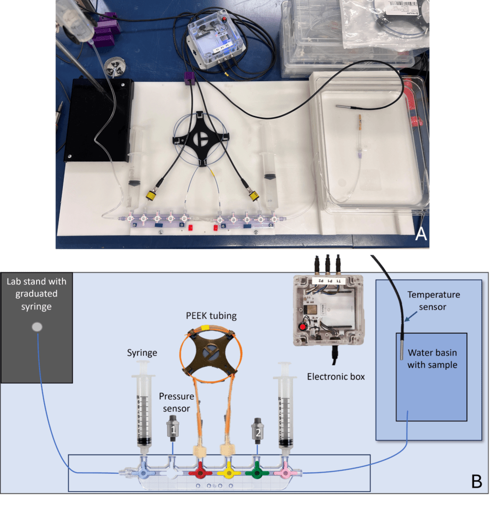
To address these issues, we developed an electronic box powered by the computer’s USB port, incorporating a low-noise supply voltage regulator. High-precision pressure transducers with a 24-bit digital output were selected to ensure reliable pressure readings across a specified pressure and temperature range (Figure 1). These transducers were calibrated and compensated over a specific temperature range for sensor offset, sensitivity, temperature effects, and nonlinearity using an application-specific integrated circuit.

Additionally, an R Shiny application was developed to simplify the process of recording hydraulic conductivity measurements.

Materials/Equipment

Supplies and equipment remain unchanged from Sack et al. (2011), except for the electronics (box, cables, pressure sensors and temperature probe). As seen in Figure 1A, the graduated cylinder was traded for an additional large syringe, and more ports can be added by extending the manifold. The additional ports can be used to connect PEEK tubing of various resistances for faster switching between tubes if necessary (e.g. measurement of samples with different conductivities).

The electronics were developed by Kynze (Saint-Bruno-de-Montarville, QC, Canada), which also recommended changing the pressure sensors to better meet our needs. These components can be purchased fully assembled by contacting Morgane Urli or assembled using the materials and instructions available on GitHub (Urli et al. 2025):

• manufacturing files with components in the pcb folder
• microcontroller code in firmware folder
• manufacturing files for the case components in the mechanical folder
• R Shiny application code files in the software folder

Units, terms, definitions

Table 1 lists the raw variables copied by the user from Arduino (Table 1). These variables serve as inputs in the R Shiny application. Table 2 lists all the variables calculated by the R Shiny application.

Table 1. Raw data extracted from Arduino during the calibration and the hydraulic conductivity measurements

Abbreviation	Variable description	Unit
ELTime	Time since start-up	s
STEP	A numerical value which is incremented using the button on the electronic box (reset by holding down the red button for one second)
P1.psi	Pressure measured by pressure sensor in position 1 (i.e. before PEEK tubing)	psi
P2.psi	Pressure measured by pressure sensor in position 2 (i.e. after PEEK tubing)	psi
T3_oC	Temperature measured by the temperature sensor	°C

 

Table 2. Data extracted from the R Shiny files after data compilation (Section 2.4)

Variable	Description	Unit
file	Name of the file associated with the measurement
parm1	Parameter to define by the user associated with the measurement (e.g. the project name)
parm2	Parameter to define by the user associated with the measurement (e.g. the operator)
parm3	Parameter to define by the user associated with the measurement (e.g. Ki vs Kmax)
parm4	Parameter to define by the user associated with the measurement (e.g. species name)
parm5	Parameter to define by the user associated with the measurement (e.g. sample identifier)
parm6	Parameter to define by the user associated with the measurement (e.g. measurement identifier)
parm7	Date of measurement
parm8	Parameter to define by the user associated with the measurement (e.g. device identifier)
VALIDPEEKCHOICE	PEEK tubing range: between 0 and 1
VALID_PEEK_TUBE	Does the PEEK tubing work between 20 and 80% of its range? OK: yes; ?: no
VALID_PSENSOR	Do pressure sensors show less than 1/1000 variation? OK: yes; RECALIBRATE: no
TIME	Was the measurement taken after 300 s? (Step 2) OK: yes; WAIT: no
STABILITY	Was the measurement stable when it was taken? (CV < 0.05) OK: yes; WAIT: no
SLOPE_P1	Slope of regression line during calibration of pressure sensor 1
INTERCEPT_P1	Intercept of the regression line during calibration of pressure sensor 1
SLOPE_P2	Slope of regression line during calibration of pressure sensor 2
INTERCEPT_P2	Intercept of the regression line during calibration of pressure sensor 2
PEEKTUBE_ID	Identifier of the PEEK tubing used during the measurement
R_PEEKTUBE_25	Resistance at 25 °C of selected PEEK tubing	MPa mmol-1 s-1
P1	Average pressure measured by pressure sensor in position 1 during measurement (Step 2)	bar
P2	Average pressure measured by pressure sensor in position 2 during measurement (Step 2)	bar
P3	Average backpressure exerted by basin water on flow	bar
K_BRUT_MMOL	Hydraulic conductance (K) without correction	mmol s-1 MPa-1
K_BRUT_KG	Hydraulic conductance (K) without correction	kg s-1 MPa-1
CV_K	Coefficient of variation of K	%
T1	Temperature of the water before measurement	°C
T2	Temperature of the water after measurement	°C
T_AV	Average T1 and T2	°C
R_PEEKTUBE_T	PEEK tubing resistance at T_AV	MPa mmol-1 s-1
T3	Average basin water temperature during the measurement	°C
K_T	K at T3 and corrected for backpressure	kg s-1 MPa-1
K_25	K at 25°C and corrected for backpressure	kg s-1 MPa-1
STEMDIAMETR_AVG	Average diameter	mm
AS	Surface	m2
STEMLENGTH	Stem length	mm
KS	Stem-specific hydraulic conductivity	kg s-1 MPa-1 m-1
COMMENTS	Comments added by the user

 

Procedure

1. The Flow Meter: From Preparation Before Measurement to Cleaning

1.1. Flow meter Preparation, solution preparation, and cleaning

Refer to Section I of Sack et al. (2011) for assembling the flow system. Ensure that the flow meter is carefully assembled, connected, secured, and filled with the appropriate solution prior to use.  Note that by using a syringe for the water column, the tubing can be screwed onto the tip to allow the solution to flow into the system (Figure 1A). Labelling with a syringe is described in Section 2.1 below.

1.2. Pressure Sensors and Electronic Box

Instructions for building the electronic box and pressure sensors needed are available on GitHub (Urli et al. 2025): The electronic box includes four outputs (Figure 1):

• 1 USB connection to the computer
• 2 pressure sensor connections (ensure correct placement; see Figure 1)
• 1 temperature sensor connection.

1.3. Cleaning the Flow Meter After Measurement

Proper cleaning of the flow meter after use is crucial to maintain the accuracy and longevity of the device. Refer to Section III of Sack et al. (2011) for detailed cleaning instructions. Ensure that all tubing and sensors are flushed with clean solution to remove any residue that could affect future measurements.

1.4. Preparing the Flow Solution and Filling the Flow Meter

Refer to Section IV of Sack et al. (2011). Handle the pressure sensors carefully to prevent shocks and excessive pressure.

 

2. Using the Flow Meter with the R Shiny Application

The raw data used in this protocol as an example can be found in the software/example folder. Additionally, a formatting section (3. Data Formatting Requirements) is included to explain the required structure of files to be copied into the application, enabling users to integrate their own data with the R Shiny application.

Clone the software repository (available on GitHub) to your local machine or download the contents.

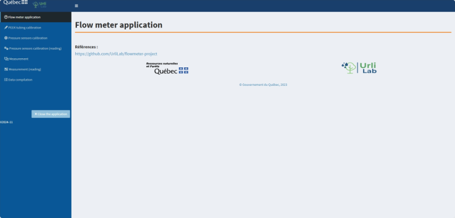
Run the ui.R script in RStudio by clicking on the Run App button, or by executing the following command in the console: shiny::runApp(‘directory/where/ui.Rfile’). The welcome interface is displayed as shown in Figure 2.

The LED (see Figure 1) on the electronic box is yellow, then green.

2.1. Determining Resistance of PEEK Tubing

This step can be performed without connecting the pressure sensors, as they are not required. It can also be completed in advance of measurement.

Before using the flow meter, it is necessary to measure the resistance of PEEK tubing used for hydraulic conductance measurements of biological material and have it stored in a calibration file.

This measurement can be done by following the procedure with a pipette described in Section V: “Determining Resistance of Peek Tubing, Temperature Correction, and Selecting the Right Tubing” of Sack et al. (2011) and using the R Shiny application. For temperatures equal to or greater than 20°C, the temperature correction for viscosity effects described in Sack et al. (2011) was considered in R Shiny. For temperatures less than 20°C, the following equation adapted from Martin and McCutcheon (1999) was used in R shiny:

where R_mes and R₂₅ are the water temperatures during the measurement (T) and corrected to 25°C, respectively.

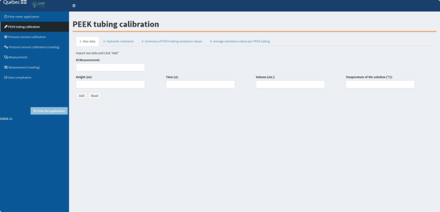
a. Click on the PEEK tubing calibration tab and on the 1- Raw data tab (Figure 3).

b. Create a unique identifier for the current PEEK tubing resistance measurement (Figure 4).

c. Add the data associated with the measurement (Table 3, Table 4) of the first water column height (Figure 4).

Table 3. Raw data for the determination of the reference resistance of PEEK tubing

Variable	Description	Unit
Height	Height of the water column	m
Duration	Duration required for water to flow through the defined volume	s
Volume	Volume	mL
T	Temperature measured by the temperature sensor in the water column	°C

d. Click Add. A table is created (Figure 5).

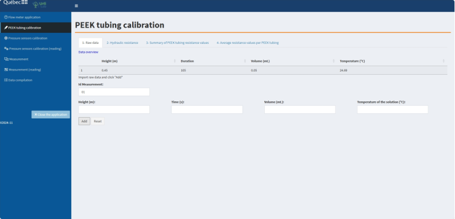
e. Repeat steps “c” and “d” for all water column heights (Figure 6). Suggested column heights (in meters) include 0.45, 0.35, 0.25, 0.15, and 0.05.

This raw data can be found in the /OUTPUTS/PEEK/measurement folder within the software directory. In the protocol example, the filename is 01_PEEKmeasurement.csv.

f. Validate the resistance data entered in 1- Raw data.

• • Click on the 2- Hydraulic resistance tab (Figure 7)

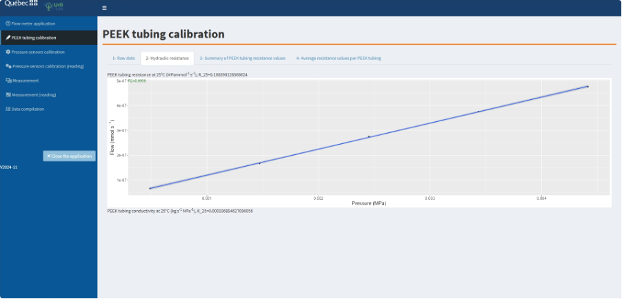
• This tab shows the relationship between flow and pressure associated with the height of the water column. For calibration to be successful, the adjusted R² value of this relationship should be greater than 0.99. If this is the case, the adjusted R² value will be written in green, and the resistance value can be kept. If the value is written in red, redo the PEEK tubing resistance measurement.

The PEEK tubing resistance value (R_25) is given in MPa mmol^-1 s^-1, which is the unit of PEEK tubing resistance used to determine the hydraulic conductivity of the biological material. This value has been corrected for temperature and therefore corresponds to the PEEK tubing resistance at 25°C.

The corresponding hydraulic conductivity at 25°C (K_25) is also given in kg s^-1 MPa^-1 in this tab.

g. Click on the 3- Summary of PEEK tubing resistance values

This tab allows the resistance values obtained in the previous tab to be saved in the file of your choice (Figure 8).

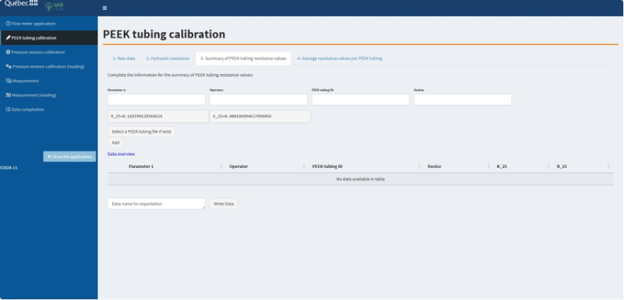
h. Complete the different parameters (i.e. Project name, Operator, PEEK tubing ID, Device), and click Add if there is no existing file to select, as is the case when using this application for the first time.

i. Name the file in which the data will be saved and click Write Data. A table is created in Data overview (Figure 9).

This file can be found in the /OUTPUTS/PEEK/id folder within the software directory. In the example of the protocol, the filename is PEEK_tubing_PEEKid.csv.

To obtain a reliable reference value for the resistance of a PEEK tubing, it is best to measure the same PEEK tubing several times and use the average resistance value for that PEEK tubing.

j. Add a new measurement for the same PEEK tubing.

• • Use the Reset button in the 1- Raw data
  • Add the raw data associated with a new measurement obtained by repeating steps “b” to “e” (Figure 6). Do not forget to use a unique measurement identifier (step “b”).
  • After step “f” validation (Figure 7), complete the 3- Summary of PEEK tubing resistance values. The parameters may be identical to the previous measurement if the same PEEK tubing was measured by the same person.
  • Click Select a PEEK tubing file if exist to add this data to an existing file (csv in our example).
  • Click Add to add the new data.

k. Name the file and click Write data. You can give it the same filename as the selected file like our example (Figure 10).

l. Click on the 4- Average resistance values per PEEK tubing tab (Figure 11).

This tab allows you to calculate the average resistance per PEEK tubing using the values previously obtained in tab 3- Summary of PEEK tubing resistance values. It creates a calibration file that can be selected when measuring the hydraulic conductance of biological materials.

m. Click Select a PEEK tubing file id and select the appropriate file. A table is created in Data overview.

n. If you want to add average resistance data to an existing file, click Select a PEEK tubing file if exist and select the appropriate file.

• • If you add to an existing file, ensure that each PEEK tubing has a unique PEEK tubing ID and that it is not already used within the file. This ID will allow you to select which PEEK tubing is attached to the system and have the correct resistance value when proceeding to measurements.

o. Click Compute mean by PEEK tubing ID and name the file (Figure 12). A new line is created in the table (Figure 14) including mean value, variance, standard deviation of PEEK tubing resistance at 25°C (MPa mmol^-1 s^-1) and hydraulic conductance at 25°C (kg s^-1 MPa^-1), and number of measurements (n).

• • Since the calculation is made by PEEK tubing ID, a calibration file can contain all PEEK tubing reference resistances of all PEEK tubing measured.

p. Click Write Data.

This file can be found in the /www/color folder within the software directory. In the example of the protocol, the filename is mean_PEEK.csv.

2.2. Pressure Sensors Calibration

The goal of the calibration is to establish a precise relationship between the water pressure, calculated based on the height of the water column (in bar) and the pressure readings from the pressure sensors (in psi). This involves constructing two separate calibration curves, one for each pressure sensor.

Calibration steps

a. Place the water column at the first graduation (5 cm).

• • Graduations should represent the difference in height between the level of the meniscus in the syringe and the level of the pressure sensors. Mark that meniscus level and where the clamp attaches to the syringe to use as references for future pressure calibrations with the same material.
  • Use tape on the dedicated lab stand to mark graduations in 5 cm increments which represent the height of the water column, from 5 cm to 50 cm. Note that these graduations will only be valid for that specific setup.
  • For a more detailed breakdown of water column height calculations, refer to Section VI: “Calibrating the Transducers” of Sack et al. (2011). The height entered in R Shiny is the water column height that we propose to label directly on the lab stand.

b. Start a measurement session by opening Arduino (Arduino > Tools > Serial Monitor). Select the appropriate COM port in Arduino if necessary.

c. Adjust the valves so that the solution flows through the sensors but does not pass through the syringes, PEEK tubing, or exit the system. The pressure measured by both sensors should correspond to the height of the water column. For further details, see Section VI: “Calibrating the Transducers” of Sack et al. (2011).

d. Hold down the red button on the electronic box (see Figure 1) for one second to ensure it is reset. Upon release, the LED will briefly turn purple before returning to green.

e. Press the red button on the electronic box. The LED changes from green to blue indicating that measurements are being recorded in Arduino.

f. Wait for at least 20 seconds (approximately 10 measurements).

g. Press the red button on the electronic again. The LED changes from blue to green, indicating the measurement process has paused.

h. Raise the water column to the next designated level (5cm above current level).

i. Press the red button on the electronic box again to increment the step and record measurements at this new level.

j. Repeat steps “e” through “i” until reaching the 50 cm graduation.

k. Press the red button on the electronic box for one second to reset it. Again, the LED will briefly turn purple before returning to green.

l. Open the Pressure sensors calibration tab in the R Shiny application and enter the required information, including the date, operator details, height levels and Arduino data (see Figure 13 and Table 5 for the formatting specifications of the Arduino data).

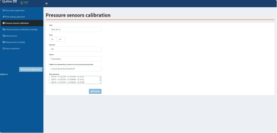
m. Click Submit.

• • If the calibration is successful, the adjusted R² of the relationship between the calculated water pressure (in bar) and the measured pressure sensor readings (in psi) should be greater than 0.99 for each pressure sensor. If this criterion is met, the boxes will turn green, and the sample can be measured (Figure 14). If the boxes turn red, inspect the system for air bubbles, verify sensors connections, and repeat the calibration process.

At the end of the calibration process, the R Shiny application will save the following data files:

• csv: raw data from the pressure and the temperature sensors (see Table 1)
• csv: summary statistics (mean, standard deviation of pressure measurements for each pressure sensor at each height level) derived from the raw data
• csv: processed calibration data, including the adjusted R² value, intercepts, and slopes of the regression relationship between the measured pressure values and the theoretical pressure values based on water column height.

These files will be stored in the /OUTPUTS/CALIBRATION folder within the software directory. In the protocol example, the filename is formatted as d_20250415_143300_MU _Flowmeter1.

2.3. Conducting Hydraulic Conductance Measurements

For sample installation in the flow meter, refer to Section VII: “Making Measurements with your Flow Meter” in Sack et al. (2011).

a. Set the water column.

• • Adjust the water column to the appropriate graduation (see Sack et al. 2011).

b. Select calibration files in R Shiny.

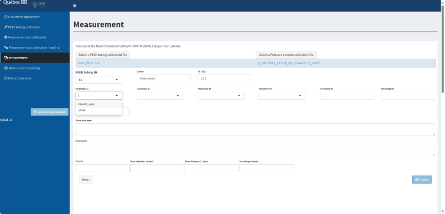
• • Click on the Measurement tab in R Shiny.
  • Select the file containing the PEEK tubing resistance values by clicking Select a PEEK tubing calibration file (see Section 2.1: “Determining resistance of Peek Tubing” for details on creating this file).
  • Select the file corresponding to the appropriate pressure sensors calibration by clicking Select a Pressure sensors calibration file.
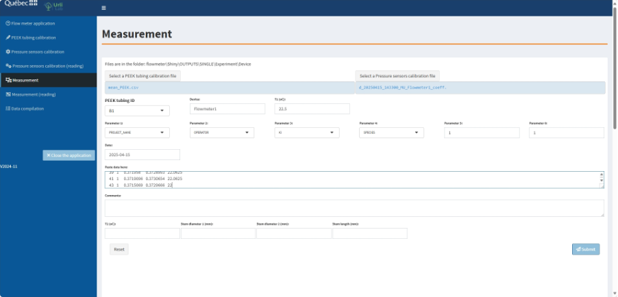
  • Fill in the required information[1]:
    1. PEEK tubing ID (same ID as in the PEEK tubing calibration file)
    2. Device
    3. Parameters 1–6 (Figure 15)

c. Measure the temperature.

• • Fully immerse the temperature probe in the water column solution.
  • Read the temperature in Arduino (Arduino > Tools > Serial Monitor).
  • Enter the value in box T1.
  • Replace the temperature probe in the ultrapure water basin containing the sample. Caution: Ensure that no water is removed from the water column during this step.

d. Reset the flow meter.

• • Before starting the measurement, ensure the flow meter has been reset. This is important so that each numerical value in the Arduino “Step” column corresponds to the respective step of measurement.
  • If needed, press the red button for one second. The LED will turn purple, then green again.

Step 1: Validation of Pressure Sensors Calibration

This quick step ensures that the pressure sensors are correctly calibrated before proceeding with sample measurement.

Procedure:

e. Position the valves.

• • Ensure that the solution flows through the sensors but not through the syringes, PEEK tubing, or out of the system.
  • The pressure measured by the two sensors should correspond to the height of the water column, as during the pressure sensors calibration.

f. Start a measurement session.

• • Measurement data should appear in Arduino. If it doesn’t, open Arduino (Arduino > Tools > Serial Monitor).

g. Initiate the measurement.

• • Press the red button on the electronic box. The LED will turn from green to blue, indicating that measurements are being recorded in Arduino.

h. Wait for data acquisition.

• • Allow a minimum of 20 seconds (equivalent to 10 measurements) to ensure stability.

i. Stop the measurement.

• • Press the red button on the electronic box again. The LED will change from blue to green, indicating that the measurement has stopped.

j. Record the results.

• • Enter the data from Step 1 into the corresponding box in the R Shiny application (Figure 16 and Table 6 for the formatting specifications of the Arduino data).

k. Submit the data.

• • Click Submit to validate the step.

• The data table cells associated with Step 1 should display “OK” and be highlighted in green, confirming that the sensor measurement variation at the same pressure is negligible (top of Figure 17).
• The average pressure measured by each sensor is displayed below in the same tab (bottom of Figure 17).
• The cells for Step 2 and the final hydraulic conductivity value remain red at this stage.
• The tab also displays:
  • Raw data from Arduino
  • Pressure sensors calibration data
  • Resistance of the selected PEEK tubing at 25°C, which will be used for sample measurement (Figure 17).
• If Step 1 is successful, proceed to Step 2, which involves measuring the sample itself.

Step 2: Sample measurement

l. Position the valves into measurement position.

• • Close the stopcocks to the syringes and open the stopcocks to the pressure sensors, the PEEK tubing and the sample.
  • The solution should flow through the sensors, the PEEK tubing, and the sample, but not through the syringes.

m. Initiate measurements.

• • Press the electronic box button. The LED should change from green to blue indicating that measurements are being taken in Arduino.

n. Wait for data acquisition for a minimum of 300 seconds.

• • This time allows measurements to stabilize and is a prerequisite for the validation of Step 2.

o. Record the results.

• • Without stopping measurements, delete the data in the box from Step 1 in R Shiny and replace it with the data from Steps 1 and 2 in Arduino.
  • Deleting Step 1 data and pasting the data from both Steps 1 and 2 reduces copy-and-paste errors that can occur by simply adding data from Step 2 into the data box.

p. Click Submit.

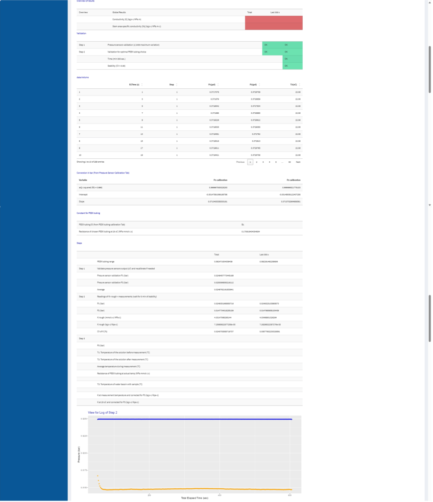
• The data table cells associated with Steps 1 and 2 should read “OK” and be highlighted in green (top of Figure 18).
• For Step 2, the cells are green if the resistance of the PEEK tubing range is comprised between 20% and 80% (59% in this example), the duration of the measurement is at least 300 s, and the coefficient of variation (CV) is < 0.05 (0.009 in this example).
• The resistance of the PEEK tubing range, the average pressure measured by each sensor during Step 2, the “rough” conductance of the sample at the actual temperature (i.e. without the correction of the backpressure exerted by the water of the sample basin, see Step 3), and the value of the CV are also indicated in this tab (Figure 18).
• The relationship between the pressure measurements of each sensor and the measurement time is also shown (bottom of Figure 18).
• The cells associated with the final hydraulic conductivity value remain red during Step 2.
• If this step is successful, press the electronic box. The LED changes from blue to green, indicating that measurement has been paused. Move on to Step 3.
• Otherwise, additional measurements can be taken to obtain a CV < 0.05. The R Shiny application performs calculations over the entire duration of Step 2 as well as over the last 300 s. The data calculated over the last 300 s are used for hydraulic conductance calculations. That is why we suggest not to stop measurement until you validate the results of Step 2 in R Shiny.

Step 3: Measurement of the backpressure exerted by the water of the sample basin

q. Position the valves to measure backpressure with pressure sensor 2.

• • Turn the stopcocks of pressure sensor 2 off to the system, so that the sensor is open only to the sample.

r. Start measurements.

• • Press the electronic box button. The LED will change from green to blue. Measurements are being taken in Arduino.

s. Wait for data acquisition for a minimum of 300 seconds.

• • Again, this time allows for stabilization of measurements.

t. Record the results.

• • Without stopping measurements, delete the data from Steps 1 and 2 in R Shiny and fill in the box with the data from Steps 1, 2, and 3 in Arduino. The same reasoning as in Step 2 applies.

u. Click Submit.

• • The relationships between the pressure measurements of each sensor (in blue for sensor 1 and orange for sensor 2) and the time of measurement are graphed (Figure 19).
  • The step is successful when the CV associated with the last 300 s measurements is < 0.05 (0.008 in this example).
  • If this step is successful, press the red button on the electronic box. The LED will change from blue to green, indicating that measurements have stopped.
  • Otherwise, as in Step 2, additional measurements can be taken to obtain a CV < 0.05. That is why we suggest that you do not stop the measurements until you have validated the results of Step 3 in R Shiny.

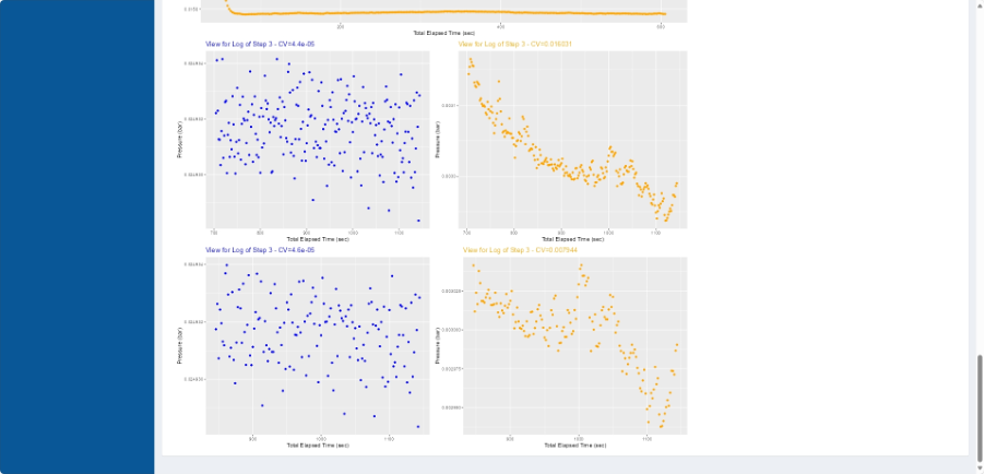
These are the last graphs at the bottom of the tab. The blue and orange dots represent data from pressure sensors 1 and 2, respectively. The graphs below show the data obtained during the last 300 s. CVs are shown above each graph. To determine whether Step 3 has been successful, the graph at the bottom right is the most useful.

v. Add comments to the Comments section if necessary.

w. Measure stem diameter.

• • Measure two diameters, one at each end of the sample (or two diameters taken perpendicularly, depending on the sample), and the length of the stem segment.
  • Enter them in R Shiny (Figure 20).
  • It is possible to adapt the R Shiny application code to an organ other than the stem if required.

x. Measure the water column final temperature.

• • Take the temperature probe and immerse it fully in the water column solution.
  • Read the temperature in Arduino (Arduino > Tools > Serial Monitor).
  • Fill in box T2.

y. Click Submit.

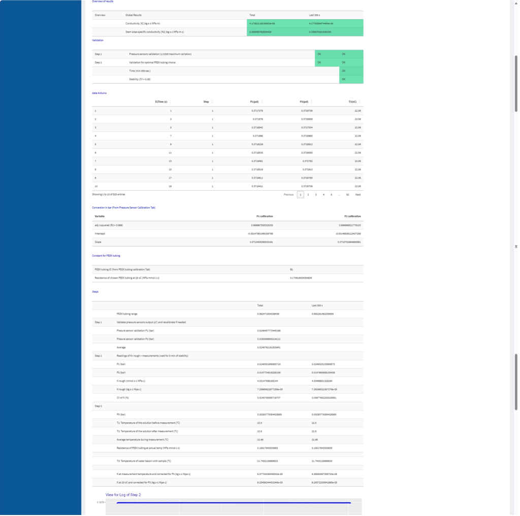
• The data table cells associated with Steps 1 and 2 and with the final hydraulic conductivity value should be highlighted in green (top of Figure 21).
• The average backpressure measured by sensor 2 (P3) during Step 3, the temperature measured before and after the measurement, the average temperature, the resistance of PEEK tubing at the actual temperature, the temperature of the water basin, the hydraulic conductance at the measurement temperature and 25°C (cf temperature correction for the viscosity effects in the 1. Determining Resistance of Peek tubing Section), the conductivity, and the stem area-specific conductivity are also indicated in this tab (Figure 21).

At the end of the sample measurement, the saved data with R Shiny are as follows:

• csv: raw data from pressure and temperature sensors (Table 1)
• csv: same table as the filename_coef.csv corresponding to the pressure sensors calibration used during the sample measurement
• csv: input created by the operator to identify the measured sample (different parameters -1 to 8- as project, species, id, comments, etc), relative to the sample (length and diameters of the sample), and its measurement (name of the file associated with the calibration, the PEEK tubing resistance value, the PEEK tubing identifier used for the measurement, temperature of the water column before and after the measurement)
• csv: PEEK tubing identifier and its hydraulic resistance at 25°C
• csv and filename_STEP.csv: analysed sample data.

These can be found in the /OUTPUTS/SINGLE/ PROJECT_NAME/DEVICE_ID folder within the software directory. In the example of the protocol, filename is PROJECT_NAME_OPERATOR_Ki_SPECIES_1_1_2025-04-15 .

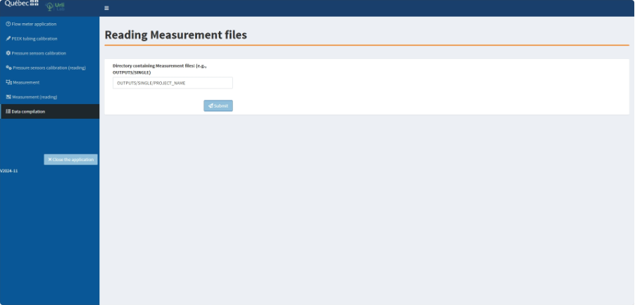
2.4. Compiling the Hydraulic Conductivity Data

The application enables data to be compiled into a single file, with each line representing a hydraulic conductivity measurement. The details of the data contained in this file are listed in Table 2.

a. Click on the Data compilation

b. Enter a path to data files (for example, OUTPUTS/SINGLE/PROJECT_NAME) (Figure 22) and click Submit.

At the end of the data compilation, the saved data files with R Shiny are as follows:

• • csv: analysed data (Table 2)
  • csv: list of input files used to build DB.csv.

These can be found in the /OUTPUTS/SINGLE/ PROJECT_NAME/OUTPUT folder within the software directory.

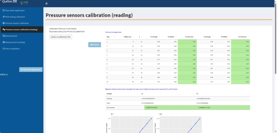
2.5. Reading Pressure Sensors Calibration and Hydraulic Conductivity Measurements

Pressure sensors calibration (reading)

The R Shiny application allows reading of the calibration files. This is useful for checking the relationships between water pressures calculated from the water column heights (in bar) and pressure readings from the pressure sensors (in psi) (Figure 23).

a. Click on the Pressure sensors calibration (reading) tab and select the appropriate file.

b. Click Submit.

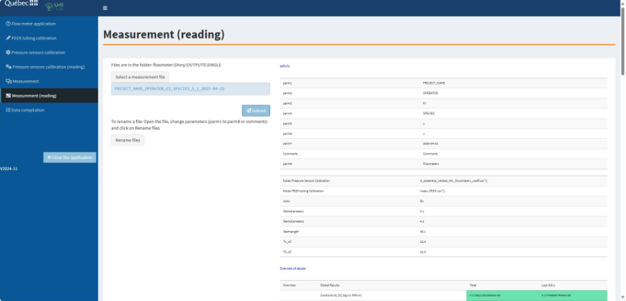
Measurements (reading)

The application also allows the measurement file to be read and the modification of parameters 1 to 8 associated with the measurement (e.g. the id of the sample, the species name).

a. Click on the Measurement (reading) tab and select the appropriate file.

b. Click Submit.

c. Double click on the parameters or Comments to change them.

d. Click Rename files to rename all files with the correct parameters (Figure 24).

• • A folder named DELETE, including all the original files, will be created, and the files with their new names and correct parameters will replace the original files.

• If you want to change variables that influenced the calculation of the hydraulic conductivity like stem length or the diameter, the measured temperature before or after the measurement or the PEEK tubing used during the measurement, we suggest you use the Measurement tab and copy-paste the data from the Arduino file associated with the measurement you want to change. Be careful: if the parameters are the same, the previous files will be overwritten.

 

3. Data Formatting Requirements

Table 4. Peek tubing resistance file formatting. Additional information on the metadata can be found in Table 3.

Height	Duration	Volume	Temperature
0.45	105	0.05	24.69
0.35	133	0.05	24.63
0.25	182	0.05	24.31
0.15	300	0.05	24.00
0.05	757	0.05	23.38

 

Table 5 Pressure sensor calibration file formatting. Additional information on the metadata can be found in Table 1.

ELTime	Step	P1.psi	P2.psi	T3_oC
1	1	0.09117617	0.09224454	21.9375
3	1	0.09154152	0.09189181	21.9375
…
32	2	0.1614722	0.1619935	21.9375
…
181	6	0.442554	0.4428779	22.1875
…
360	10	0.7247037	0.7248018	22.3125

 

Table 6 Sample measurement file formatting. Additional information on the metadata can be found in Table 1.

ELTime	Step	P1.psi	P2.psi	T3_oC
1	1	0.3717078	0.3726709	22.0625
3	1	0.371879	0.3728859	22.0625
…
53	2	0.3714092	0.2560349	22
55	2	0.3718674	0.2463562	22.0625
…
704	3	0.3717332	0.06527864	21.8125
…
1144	3	0.3717421	0.06311297	21.75

 

Notes and troubleshooting tips

We also developed a structure that supports the water column, the water basin, the manifolds and the pressure sensors to standardize our different devices. Contact Morgane Urli for further details.

Do not forget to follow the recommendations of Sack et al. (2011) to clean the flow meter.

 

Links to resources and suppliers

https://github.com/UrliLab/flowmeter-project

 

Literature references

Chang W, Cheng J, Allaire J, Sievert C, Schloerke B, Xie Y, Allen J, McPherson J, Dipert A, Borges B (2024). _shiny: Web Application Framework for R_. R package version 1.9.1, https://CRAN.R-project.org/package=shiny

Melcher PJ., Holbrook MN, Burns MJ, Zwieniecki MA, Cobb AR, Brodribb TJ, Choat B, Sack L (2012) Measurements of stem xylem hydraulic conductivity in the laboratory and field. Methods in Ecology and Evolution 3(4), 685–694. https://doi.org/10.1111/j.2041-210X.2012.00204.x

Martin JL and McCutcheon SC (1999). Hydrodynamics and Transport for Water Quality Modeling, 1st edition. ed. CRC Press, Boca Raton. https://doi.org/10.1201/9780203751510

R Core Team (2024). _R: A Language and Environment for Statistical Computing_. R Foundation for Statistical Computing, Vienna, Austria. <https://www.R-project.org/&gt;. “R version 4.4.1 (2024-06-14 ucrt)”

Sack L, Bartlett MK, Creese C, Guyot G, Scoffoni C, contributors (2011). Constructing and operating a hydraulic flow meter: PrometheusWiki. http://prometheuswiki.org/tiki-index.php?page=Constructing+and+operating+a+hydraulics+flow+meter.

Urli M., Lambert M.-C., and Périé C. (2025). UrliLab/flowmeter-project: v1.3. Version 1.3, https://doi.org/10.5281/zenodo.16969363

 

Acknowledgments 

We would like to express our sincere gratitude to Linda Veilleux (MRNF) and Daniel Girard (MRNF) for their foundational work on designing the first version of the device. Our heartfelt thanks go to Karine Thériault (MRNF) and Katherine Galibois (MRNF) for their significant contributions to developing the most recent iteration of the apparatus. We also extend our appreciation to Kynze for their role in developing the electronic casings and pressure sensors.

We are grateful to Katherine Galibois, Karine Thériault, Thomas Villeneuve (UQAM), Maya Mignot (UQAM), and Audrey Bédard (UQAM) for their dedication in updating the laboratory protocols over the years. Additionally, we thank Jessica Samson-Tshimbalanga (MRNF) for her careful revision and harmonization of the final version of the protocol.

We would also like to thank Ellie Nichols for her thoughtful review and constructive feedback on the manuscript, which helped improve its clarity and structure.

This project was made possible thanks to the financial support of the Government of Québec through the Fonds Vert du Québec and Plan pour une économie verte 2030.

[1] The dropdown menus for parameters 1–4 can be customized by modifying the parm_choice.csv file in the software/www folder. It should be done before starting the R Shiny application for the menus to be updated. In the example:

• Parameter 1: Research project name
• Parameter 2: Operator name/initials
• Parameter 3: Measurement type (e.g., initial or maximum conductance after embolism removal)
• Parameter 4: Species
• Parameter 5 & 6: Individual ID and measurement ID (if multiple measurements are taken on the same individual).