 Protocol
Author
Kenji Omasa – aomasa@mail.ecc.u-tokyo.ac.jp
Summary
Imaging techniques such as multispectral and hyperspectral imaging, thermal imaging, fluorescence imaging, and computed tomography have been widely used for plant functional analysis from cells to whole plants (e.g. Omasa 1990; Papageorgiou and Govindjee 2004; Jones and Morison 2007; Furbank 2009; Simpson et al. 2011). Two-dimensional (2D) digital imaging of chlorophyll fluorescence quenching is one of the leading methods used to assess photosynthetic activities in leaves (Omasa et al. 1987; Daley et al 1989; Genty and Mayer 1995) and at cellular levels (Oxborough and Baker 1997). Recent advance in chlorophyll fluorescence imaging is three-dimensional (3D) analysis of whole plant (Omasa et al. 2007; Konishi et al. 2009) and at cellular levels (Endo and Omasa 2007; Omasa et al. 2009). Combined chlorophyll fluorescence and thermal imaging is useful for analysis of relationships between photochemical and non-photochemical quenching and stomatal response (Omasa and Takayama 2003; Omasa et al, 2007). In this section, several chlorophyll fluorescence imaging techniques are introduced.
2D imaging of chlorophyll fluorescence during dark-light transition
This imaging technique is suitable for analysing Kautsky effect and steady-state fluorescence (Omasa et al. 1987). Lighting system (e.g. LEDs and metal halide lamp equipped with a short pass heat absorbing filter and fibre optics) is used to uniformly illuminate actinic light of wavelength from 400 nm to 680nm on attached leaves for photosynthesis. After dark adaptation about 20 min., light intensity (PPF) on the leaves is changed from 0 μmol m-2 s-1 to the desired actinic light intensity. Changes in chlorophyll a fluorescence images are captured using a high-resolution wide dynamic range video camera equipped with a band pass filter within a range of 680 to 750nm and analysed by a computer.
2D imaging of non-photochemical quenching and photochemical yield of photosystem
Non-photochemical quenching (NPQ) and photochemical yield of photosystem ( PS ) are calculated from a set of chlorophyll fluorescence images captured using the above-mentioned band-pass video camera under combinations of the actinic light for photosynthesis and saturation light pulse (several thousands μmol m-2s-1 for 2 s) that caused a transient saturation of photochemistry. Using the relative fluorescence yield images, NPQ and PS images are computed for each corresponding pixel using the following equations (Daley et al 1989; Genty and Mayer 1995; Omasa and Takayama 2003)
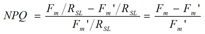
and

where, Fm is the chlorophyll fluorescence intensity measured during a saturation light pulse (about 2s) after dark adaptation for at least 20min, F is the chlorophyll fluorescence intensity measured under the steady-state actinic light, Fm‘ is the chlorophyll fluorescence intensity measured during the saturation light pulse (about 2 s) just after Fm‘ measurement, RSL is the saturation light pulse intensity, and RAL is the actinic light intensity. The NPQ image, ranging from 0 to infinity, represents the extent of intrathylakoid pH gradient and the ability of chloroplasts to dissipate excess excitation energy as heat (Bilger and Björkman 1990; Maxwell & Johnson 2000). The PS image obtained under actinic light represents the activity of linear electron transport in PS and ranged from 0 to 1 (Genty et al. 1989; Maxwell & Johnson 2000 ).
Combined 3D range and chlorophyll fluorescence imaging
3D chlorophyll fluorescence image of whole plants is produced by combining with 3D range imaging (Omasa et al. 2007; Konishi et al. 2009). High-resolution portable scanning lidar and multi-camera stereo system are used for 3D range imaging of whole plants. The range data obtained from different measuring points are co-registered into the same orthogonal coordinates as a triangle-polygon image after noise exclusion. Consequently, each leaf was created as a polygon shell in the 3D polygon model (3D range image). After then, the chlorophyll fluorescence images are mapped on the 3D polygon model of whole plants by a texture-mapping technique. Through the correspondence of the coordinates of 2D image to 3D polygon model, the information of 2D image is automatically mapped onto each polygon shell of the 3D polygon model.
Chlorophyll fluorescence microscopy with ordinary light microscope
Chlorophyll fluorescence microscopy is an advanced technique in chlorophyll fluorescence imaging to noninvasively detect spatiotemporal changes in photosynthetic activities at the level of tissues, individual cells and chloroplasts. Ordinary 2D chlorophyll fluorescence microscopy is achieved by imaging Fm, Fm’ and F using a light microscope and computing NPQ and PS (Oxborough and Baker 1997). Therefore, it is important to measure precisely the actinic light and saturation light pulse intensities, Fm, Fm’ and F on the leaf tissues attached to light microscope stage. In 3D surface microscopy of chlorophyll fluorescence, extended-focus PS images of the leaf tissue and cell surface are reconstructed from about 15 images of chlorophyll fluorescence measured at different focal planes using shape-from-focus method (Endo and Omasa 2007). Despite the highly efficient methods for reconstruction, the internal 3D anatomy of tissues and cells is not visualized, as the 3D surface reconstruction is performed passively.
3D chlorophyll fluorescence microscopy with high-speed rotating pinhole disk CLSM
Computer-aided chlorophyll fluorescence imaging system with modified high-speed rotating pinhole disk (Nipkow disk) CLSM provides the internal 3D information on photosynthesis of leaf tissue-, cell- and chloroplast-levels (Omasa et al. 2009). This system consists of an inverted light microscope, a confocal scanner unit, a 488-nm-wavelength laser diode system, a highly sensitive cooled EM-CCD camera, various controlling devices, and a personal computer. To measure chlorophyll fluorescence, a long-pass filter (wavelength>515 nm) is built into the confocal scanner unit. For precise and rapid control of the objective position a piezo z-scan unit with 10 nm resolution and 30 ms scan rate is used. Series of chlorophyll fluorescence intensity images (Fm, Fm‘ and F ) are captured with the EM-CCD camera at different 64 focal planes within 2s. After calibrating dark current, 3D- PSII image and NPQ values are calculated from the series of chlorophyll fluorescence intensity images.
Literature references
Bilger W, Björkman O (1990) Role of the xanthophyll cycle in photoprotection elucidated by measurements of light-induced absorbency changes, fluorescence and photosynthesis in leaves of Hedera canariensis. Photosynthesis Research 25:173-185.
Daley PF, Raschke K, Ball JT, Berry JA (1989) Topography of photosynthetic activity of leaves obtained from video images of chlorophyll fluorescence. Plant Physiology 90:1233-1238.
Endo R, Omasa K (2007) 3-D cell-level chlorophyll fluorescence imaging of ozone-injured sunflower leaves using a new passive light microscope system. Journal of Experimental Botany 58:765-772.
Furbank RT (ed) (2009) -Plant phenomics’ Functional Plant Biology. 36:845-1126
Genty B, Meyer S (1995) Quantitative mapping of leaf photosynthesis using chlorophyll fluorescence imaging. Australian Journal of Plant Physiology 22:277-284.
Genty B, Briantais JM, Baker NR (1989) The relationship between the quantum yield of photosynthetic electron-transport and quenching chlorophyll fluorescence. Biochimica et Biophysica Acta. 990:87-92.
Jones H G, Morison J (eds) (2007) -Imaging stress responses in plants’ Journal of Experimental. Botany 58:743-898.
Konishi A, Eguchi A, Hosoi F, Omasa K (2009) 3D monitoring spatio-temporal effects of herbicide on a whole plant using combined range and chlorophyll a fluorescence imaging. Functional Plant Biology 36:874-879
Maxwell K, Johnson GN (2000) Chlorophyll fluorescence – a practical guide. Journal of Experimental Botany 51:659-668.
Omasa K (1990) Image instrumentation methods of plant analysis. In –Modern methods of plant analysis. New series Vol.11 (EdsHF Linskens,JF Jackson) pp. 203-243. (Springer-Verlag: Berlin)
Omasa K, Takayama K (2003) Simultaneous measurement of stomatal conductance, non-photochemical quenching, and photochemical yield of photosystem II in intact leaves by thermal and chlorophyll fluorescence imaging. Plant and Cell Physiology 44:1290-1300.
Omasa K, Hosoi F, Konishi A (2007) 3D lidar imaging for detecting and understanding plant responses and canopy structure. Journal of Experimental Botany 58:881-898.
Omasa K, Konishi A, Tamura H, Hosoi F (2009) 3D confocal laser scanning microscopy for the analysis of chlorophyll fluorescence parameters of chloroplasts in intact leaf tissues. Plant and Cell Physiology 50, 90-105.
Omasa K, Shimazaki K, Aiga I, Larcher W, Onoe M (1987) Imageanalysis of chlorophyll fluorescence transients for diagnosing the photosynthetic system of attached leaves. Plant Physiology 84, 748-752.
Oxborough K, Baker NR (1997) An instrument capable of imaging chlorophyll a fluorescence from intact leaves at very low irradiance and at cellular and subcellular levels of organization. Plant, Cell and Environment 20:1473-1483.
Papageorgiou GC, Govindjee (eds) (2004) Advances in photosynthesis and respiration Vol.19: Chlorophyll a fluorescence: A signiture of photosynthesis. (Springer:Dordrecht)
Simpson AJ, McNally DJ, Simpson MJ (2011) NMR spectroscopy in environmental research: From molecular interactions to global processes. Progress in Nuclear Magnetic Resonance Spectroscopy 58 :97-175